Analyzing TCR data
[1]:
# new function to setup tutorial data
from dandelion.tutorial import setup_dandelion_tutorial_tcr

setup_dandelion_tutorial_tcr()

# change to the tutorial data directory
import os

os.chdir("dandelion_tutorial")
I’m showing two examples for reading in the data: with or without reannotation.
Read in AIRR format
[2]:
import dandelion as ddl

# read in the airr_rearrangement.tsv file
file1 = "sc5p_v2_hs_PBMC_10k_t/airr_rearrangement.tsv"
file2 = "sc5p_v1p1_hs_melanoma_10k_t/airr_rearrangement.tsv"
[3]:
vdj1 = ddl.read_10x_airr(file1)
vdj1
[3]:
Lazy Dandelion object with n_obs = 5351 and n_contigs = 10860
    data: cell_id, sequence_id, sequence, sequence_aa, productive, rev_comp, v_call, v_cigar, d_call, d_cigar, j_call, j_cigar, c_call, c_cigar, sequence_alignment, germline_alignment, junction, junction_aa, junction_length, junction_aa_length, v_sequence_start, v_sequence_end, d_sequence_start, d_sequence_end, j_sequence_start, j_sequence_end, c_sequence_start, c_sequence_end, consensus_count, umi_count, is_cell, locus, rearrangement_status
    metadata: cell_id, productive_VDJ, productive_VJ, v_call_VDJ, v_call_VJ, d_call_VDJ, j_call_VDJ, j_call_VJ, c_call_VDJ, c_call_VJ, junction_VDJ, junction_VJ, junction_aa_VDJ, junction_aa_VJ, locus_VDJ, locus_VJ, umi_count_VDJ, umi_count_VJ, productive_VDJ_main, productive_VJ_main, v_call_VDJ_main, v_call_VJ_main, d_call_VDJ_main, j_call_VDJ_main, j_call_VJ_main, c_call_VDJ_main, c_call_VJ_main, junction_VDJ_main, junction_VJ_main, junction_aa_VDJ_main, junction_aa_VJ_main, locus_VDJ_main, locus_VJ_main, umi_count_VDJ_main, umi_count_VJ_main, locus_status, chain_status, rearrangement_status_VDJ, rearrangement_status_VJ
[4]:
vdj2 = ddl.read_10x_airr(file2)
vdj2
[4]:
Lazy Dandelion object with n_obs = 1560 and n_contigs = 2755
    data: cell_id, sequence_id, sequence, sequence_aa, productive, rev_comp, v_call, v_cigar, d_call, d_cigar, j_call, j_cigar, c_call, c_cigar, sequence_alignment, germline_alignment, junction, junction_aa, junction_length, junction_aa_length, v_sequence_start, v_sequence_end, d_sequence_start, d_sequence_end, j_sequence_start, j_sequence_end, c_sequence_start, c_sequence_end, consensus_count, umi_count, is_cell, locus, rearrangement_status
    metadata: cell_id, productive_VDJ, productive_VJ, v_call_VDJ, v_call_VJ, d_call_VDJ, j_call_VDJ, j_call_VJ, c_call_VDJ, c_call_VJ, junction_VDJ, junction_VJ, junction_aa_VDJ, junction_aa_VJ, locus_VDJ, locus_VJ, umi_count_VDJ, umi_count_VJ, productive_VDJ_main, productive_VJ_main, v_call_VDJ_main, v_call_VJ_main, d_call_VDJ_main, j_call_VDJ_main, j_call_VJ_main, c_call_VDJ_main, c_call_VJ_main, junction_VDJ_main, junction_VJ_main, junction_aa_VDJ_main, junction_aa_VJ_main, locus_VDJ_main, locus_VJ_main, umi_count_VDJ_main, umi_count_VJ_main, locus_status, chain_status, rearrangement_status_VDJ, rearrangement_status_VJ
[5]:
# combine into a singular object
# let's add the sample_id to each cell barcode so that we don't end up overlapping later on
vdj1.add_cell_prefix("sc5p_v2_hs_PBMC_10k_t_")
vdj2.add_cell_prefix("sc5p_v1p1_hs_melanoma_10k_t_")

# combine into a singular object
vdj = ddl.tl.concat([vdj1, vdj2])
vdj
[5]:
Lazy Dandelion object with n_obs = 6911 and n_contigs = 13615
    data: cell_id, sequence_id, sequence, sequence_aa, productive, rev_comp, v_call, v_cigar, d_call, d_cigar, j_call, j_cigar, c_call, c_cigar, sequence_alignment, germline_alignment, junction, junction_aa, junction_length, junction_aa_length, v_sequence_start, v_sequence_end, d_sequence_start, d_sequence_end, j_sequence_start, j_sequence_end, c_sequence_start, c_sequence_end, consensus_count, umi_count, is_cell, locus, rearrangement_status
    metadata: cell_id, productive_VDJ, productive_VJ, v_call_VDJ, v_call_VJ, d_call_VDJ, j_call_VDJ, j_call_VJ, c_call_VDJ, c_call_VJ, junction_VDJ, junction_VJ, junction_aa_VDJ, junction_aa_VJ, locus_VDJ, locus_VJ, umi_count_VDJ, umi_count_VJ, productive_VDJ_main, productive_VJ_main, v_call_VDJ_main, v_call_VJ_main, d_call_VDJ_main, j_call_VDJ_main, j_call_VJ_main, c_call_VDJ_main, c_call_VJ_main, junction_VDJ_main, junction_VJ_main, junction_aa_VDJ_main, junction_aa_VJ_main, locus_VDJ_main, locus_VJ_main, umi_count_VDJ_main, umi_count_VJ_main, locus_status, chain_status, rearrangement_status_VDJ, rearrangement_status_VJ
Read in with reannotation
We specify the filename_prefix option because they have different prefixes that precedes _contig.fasta and _contig_annotations.csv.
[6]:
samples = ["sc5p_v2_hs_PBMC_10k_t", "sc5p_v1p1_hs_melanoma_10k_t"]

ddl.pp.format_fastas(samples, prefix=samples, filename_prefix="filtered")
Formatting fasta(s) : 100%|██████████| 2/2 [00:01<00:00, 1.12it/s]
Make sure to toggle loci = 'tr' for TCR data. I’m setting reassign_dj = True so as to try and force a reassignment of J genes (and D genes if it can) with stricter cut offs.
[7]:
ddl.pp.reannotate_genes(
    samples, loci="tr", reassign_dj=True, filename_prefix="filtered"
)
Assigning genes : 0%| | 0/2 [00:00<?, ?it/s]
         START> MakeDB
       COMMAND> igblast
  ALIGNER_FILE> filtered_contig_igblast.fmt7
      SEQ_FILE> filtered_contig.fasta
         NPROC> 8
       ASIS_ID> False
    ASIS_CALLS> False
      VALIDATE> strict
      EXTENDED> True
INFER_JUNCTION> False

PROGRESS> 16:36:02 |Done                | 0.0 min

PROGRESS> 16:36:13 |####################| 100% (13,630) 0.2 min

OUTPUT> filtered_contig_igblast_db-pass.tsv
  PASS> 12246
  FAIL> 1384
   END> MakeDb

         START> MakeDB
       COMMAND> igblast
  ALIGNER_FILE> filtered_contig_igblast.fmt7
      SEQ_FILE> filtered_contig.fasta
         NPROC> 8
       ASIS_ID> False
    ASIS_CALLS> False
      VALIDATE> strict
      EXTENDED> True
INFER_JUNCTION> False

PROGRESS> 16:36:15 |Done                | 0.0 min

PROGRESS> 16:36:24 |####################| 100% (13,630) 0.1 min

OUTPUT> filtered_contig_igblast_db-pass.tsv
  PASS> 12246
  FAIL> 1384
   END> MakeDb
Assigning genes : 50%|█████ | 1/2 [04:54<04:54, 294.36s/it]
         START> MakeDB
       COMMAND> igblast
  ALIGNER_FILE> filtered_contig_igblast.fmt7
      SEQ_FILE> filtered_contig.fasta
         NPROC> 8
       ASIS_ID> False
    ASIS_CALLS> False
      VALIDATE> strict
      EXTENDED> True
INFER_JUNCTION> False

PROGRESS> 16:38:06 |Done                | 0.0 min

PROGRESS> 16:38:11 |####################| 100% (3,706) 0.1 min

OUTPUT> filtered_contig_igblast_db-pass.tsv
  PASS> 3217
  FAIL> 489
   END> MakeDb

         START> MakeDB
       COMMAND> igblast
  ALIGNER_FILE> filtered_contig_igblast.fmt7
      SEQ_FILE> filtered_contig.fasta
         NPROC> 8
       ASIS_ID> False
    ASIS_CALLS> False
      VALIDATE> strict
      EXTENDED> True
INFER_JUNCTION> False

PROGRESS> 16:38:12 |Done                | 0.0 min

PROGRESS> 16:38:16 |####################| 100% (3,706) 0.1 min

OUTPUT> filtered_contig_igblast_db-pass.tsv
  PASS> 3217
  FAIL> 489
   END> MakeDb
Assigning genes : 100%|██████████| 2/2 [06:35<00:00, 197.78s/it]
There’s no need to run the the rest of the preprocessing steps.
We’ll read in the reannotated files like as follow:
[8]:
import pandas as pd

tcr_files = []
for sample in samples:
    file_location = sample + "/dandelion/filtered_contig_dandelion.tsv"
    tcr_files.append(pd.read_csv(file_location, sep="\t"))
tcr = pd.concat(tcr_files, ignore_index=True)
tcr.reset_index(inplace=True, drop=True)
tcr
[8]:
| sequence_id | sequence | rev_comp | productive | v_call | d_call | j_call | sequence_alignment | germline_alignment | junction | ... | d_germline_alignment_blastn | d_call_igblastn | d_source | d_support_igblastn | d_score_igblastn | j_call_multimappers | j_call_multiplicity | j_call_sequence_start_multimappers | j_call_sequence_end_multimappers | j_call_support_multimappers | |
|---|---|---|---|---|---|---|---|---|---|---|---|---|---|---|---|---|---|---|---|---|---|
| 0 | sc5p_v2_hs_PBMC_10k_t_AAACCTGAGCGATAGC_contig_1 | CTGGAAGACCACCTGGGCTGTCATTGAGCTCTGGTGCCAGGAGGAA... | F | T | TRAV23/DV6*02 | NaN | TRAJ22*01 | CAGCAGCAGGTGAAACAAAGTCCTCAATCTTTGATAGTCCAGAAAG... | CAGCAGCAGGTGAAACAAAGTCCTCAATCTTTGATAGTCCAGAAAG... | TGTGCAGCAAGCAAGGGTTCTGCAAGGCAACTGACCTTT | ... | NaN | NaN | NaN | NaN | NaN | ["TRAJ22*01"] | 1 | [412] | [466] | [2.61e-25] |
| 1 | sc5p_v2_hs_PBMC_10k_t_AAACCTGAGCGATAGC_contig_2 | GAGAGTCCTGCTCCCCTTTCATCAATGCACAGATACAGAAGACCCC... | F | T | TRBV6-5*01 | NaN | TRBJ2-3*01 | AATGCTGGTGTCACTCAGACCCCAAAATTCCAGGTCCTGAAGACAG... | AATGCTGGTGTCACTCAGACCCCAAAATTCCAGGTCCTGAAGACAG... | TGTGCCAGCAGTTACCGGGGGGGATCGGAAGATACGCAGTATTTT | ... | NaN | NaN | NaN | NaN | NaN | ["TRBJ2-3*01"] | 1 | [423] | [466] | [3.47e-19] |
| 2 | sc5p_v2_hs_PBMC_10k_t_AAACCTGAGTCACGCC_contig_2 | CCTTTTCACCAATGCACAGACCCAGAGGACCCCTCCATCCTGCAGT... | F | T | TRBV6-2*01,TRBV6-3*01 | NaN | TRBJ2-6*01 | AATGCTGGTGTCACTCAGACCCCAAAATTCCGGGTCCTGAAGACAG... | AATGCTGGTGTCACTCAGACCCCAAAATTCCGGGTCCTGAAGACAG... | TGTGCCAGCAGTTATCTCCCCCGTAGACAGGACAGGGAATCCTCTG... | ... | NaN | NaN | NaN | NaN | NaN | ["TRBJ2-6*01"] | 1 | [422] | [474] | [3.5e-24] |
| 3 | sc5p_v2_hs_PBMC_10k_t_AAACCTGAGTCACGCC_contig_1 | GTAGCTCGTTGATATCTGTGTGGATAGGGAGCTGTGACGAGGGCAA... | F | T | TRAV8-6*02 | NaN | TRAJ8*01 | GCCCAGTCTGTGACCCAGCTTGACAGCCAAGTCCCTGTCTTTGAAG... | GCCCAGTCTGTGACCCAGCTTGACAGCCAAGTCCCTGTCTTTGAAG... | TGTGCTGTGAGTGCGTTTTTTCAGAAACTTGTATTT | ... | NaN | NaN | NaN | NaN | NaN | ["TRAJ8*01"] | 1 | [566] | [614] | [7.35e-22] |
| 4 | sc5p_v2_hs_PBMC_10k_t_AAACCTGCACGTCAGC_contig_1 | CCCACATGAAGTGTCTACCTTCTGCAGACTCCAATGGCTCAGGAAC... | F | T | TRAV1-2*01 | NaN | TRAJ33*01 | GGACAAAACATTGACCAG...CCCACTGAGATGACAGCTACGGAAG... | GGACAAAACATTGACCAG...CCCACTGAGATGACAGCTACGGAAG... | TGTGCTGTCATGGATAGCAACTATCAGTTAATCTGG | ... | NaN | NaN | NaN | NaN | NaN | ["TRAJ33*01"] | 1 | [407] | [463] | [2.01e-26] |
| ... | ... | ... | ... | ... | ... | ... | ... | ... | ... | ... | ... | ... | ... | ... | ... | ... | ... | ... | ... | ... | ... |
| 15458 | sc5p_v1p1_hs_melanoma_10k_t_TTTGGTTTCACAGGCC_c... | AATGGCTCAGGAACTGGGAATGCAGTGCCAGGCTCGTGGTATCCTG... | F | T | TRAV1-2*01 | NaN | TRAJ20*01 | GGACAAAACATTGACCAG...CCCACTGAGATGACAGCTACGGAAG... | GGACAAAACATTGACCAG...CCCACTGAGATGACAGCTACGGAAG... | TGTGCTGTGATGGGGGACTACAAGCTCAGCTTT | ... | NaN | NaN | NaN | NaN | NaN | ["TRAJ20*01"] | 1 | [380] | [428] | [5.22e-22] |
| 15459 | sc5p_v1p1_hs_melanoma_10k_t_TTTGGTTTCTTTACGT_c... | TTCCTCTGCTCTGGCAGCAGATCTCCCAGAGGGAGCAGCCTGACCA... | F | T | TRBV30*01 | NaN | TRBJ2-5*01 | TCTCAGACTATTCATCAATGGCCAGCGACCCTGGTGCAGCCTGTGG... | TCTCAGACTATTCATCAATGGCCAGCGACCCTGGTGCAGCCTGTGG... | TGTGCCTGGAGTGAGCTAGCGGCCCAAGAGACCCAGTACTTC | ... | NaN | NaN | NaN | NaN | NaN | ["TRBJ2-5*01"] | 1 | [457] | [503] | [8.02e-21] |
| 15460 | sc5p_v1p1_hs_melanoma_10k_t_TTTGGTTTCTTTACGT_c... | GATCTTAATTGGGAAGAACAAGGATGACATCCATTCGAGCTGTATT... | F | F | TRAV13-1*02 | NaN | TRAJ43*01 | GGAGAGAATGTGGAGCAGCATCCTTCAACCCTGAGTGTCCAGGAGG... | GGAGAGAATGTGGAGCAGCATCCTTCAACCCTGAGTGTCCAGGAGG... | TGTGCAGCAAGTACAACCCGAAGGTTAGGCGGGGTGGGGTCAAAAA... | ... | NaN | NaN | NaN | NaN | NaN | ["TRAJ43*01"] | 1 | [388] | [439] | [2.49e-20] |
| 15461 | sc5p_v1p1_hs_melanoma_10k_t_TTTGTCACATTTCACT_c... | TCTGGGGATGTTCACAGAGGGCCTGGTCTGGAATATTCCACATCTG... | F | T | TRBV12-4*01 | NaN | TRBJ1-1*01 | GATGCTGGAGTTATCCAGTCACCCCGGCACGAGGTGACAGAGATGG... | GATGCTGGAGTTATCCAGTCACCCCGGCACGAGGTGACAGAGATGG... | TGTGCCAGCAGTTTAGGATGGGGAGACGGCACTGAAGCTTTCTTT | ... | NaN | NaN | NaN | NaN | NaN | ["TRBJ1-1*01"] | 1 | [419] | [462] | [3.45e-19] |
| 15462 | sc5p_v1p1_hs_melanoma_10k_t_TTTGTCACATTTCACT_c... | AGATCAGAAGAGGAGGCTTCTCACCCTGCAGCAGGGACCTGTGAGC... | F | T | TRAV38-2/DV8*01 | NaN | TRAJ32*01,TRAJ32*02 | GCTCAGACAGTCACTCAGTCTCAACCAGAGATGTCTGTGCAGGAGG... | GCTCAGACAGTCACTCAGTCTCAACCAGAGATGTCTGTGCAGGAGG... | TGTGCTTATAGGAGCACCCAGATCCCCCAGCTCATCTTT | ... | NaN | NaN | NaN | NaN | NaN | ["TRAJ32*02"] | 1 | [408] | [449] | [4.25e-18] |
15463 rows × 96 columns
The reannotated file can be used with dandelion as per the BCR tutorial.
For the rest of the tutorial, I’m going to show how to proceed with 10x’s AIRR format file instead as there are some minor differences.
Import modules for use with scanpy
[9]:
import anndata as ad
import scanpy as sc

import warnings

warnings.filterwarnings("ignore")
sc.logging.print_header()
[9]:
Import the transcriptome data
[10]:
adata_list = []
for sample in samples:
    adata_tmp = sc.read_10x_h5(
        f"{sample}/filtered_feature_bc_matrix.h5", gex_only=True
    )
    adata_tmp.obs["sample_id"] = sample
    adata_tmp.obs_names = [sample + "_" + x for x in adata_tmp.obs_names]
    adata_tmp.var_names_make_unique()
    adata_list.append(adata_tmp)
adata = ad.concat(adata_list)
adata
[10]:
AnnData object with n_obs × n_vars = 17275 × 36601
    obs: 'sample_id'
Run QC on the transcriptome data.
[11]:
ddl.pp.recipe_scanpy_qc(adata)
adata
OMP: Info #276: omp_set_nested routine deprecated, please use omp_set_max_active_levels instead.
[11]:
AnnData object with n_obs × n_vars = 17275 × 36601
    obs: 'sample_id', 'n_genes', 'n_genes_by_counts', 'total_counts', 'total_counts_mt', 'pct_counts_mt', 'scrublet_score', 'is_doublet', 'filter_rna'
Filtering TCR data.
Note that I’m using the Dandelion object as input rather than the pandas dataframe (yes both types of input will works. In fact, a file path to the .tsv will work too).
[12]:
adata.obs
[12]:
| sample_id | n_genes | n_genes_by_counts | total_counts | total_counts_mt | pct_counts_mt | scrublet_score | is_doublet | filter_rna | |
|---|---|---|---|---|---|---|---|---|---|
| sc5p_v2_hs_PBMC_10k_t_AAACCTGAGACAGACC-1 | sc5p_v2_hs_PBMC_10k_t | 1982 | 1982 | 4751.0 | 202.0 | 4.251737 | 0.000279 | False | False |
| sc5p_v2_hs_PBMC_10k_t_AAACCTGAGCGATAGC-1 | sc5p_v2_hs_PBMC_10k_t | 1761 | 1761 | 5767.0 | 111.0 | 1.924744 | 0.000279 | False | False |
| sc5p_v2_hs_PBMC_10k_t_AAACCTGAGCGGCTTC-1 | sc5p_v2_hs_PBMC_10k_t | 1957 | 1957 | 4991.0 | 125.0 | 2.504508 | 0.000279 | False | False |
| sc5p_v2_hs_PBMC_10k_t_AAACCTGAGGATCGCA-1 | sc5p_v2_hs_PBMC_10k_t | 2310 | 2310 | 6012.0 | 222.0 | 3.692615 | 0.000279 | False | False |
| sc5p_v2_hs_PBMC_10k_t_AAACCTGAGTCACGCC-1 | sc5p_v2_hs_PBMC_10k_t | 2315 | 2315 | 7267.0 | 158.0 | 2.174212 | 0.000279 | False | False |
| ... | ... | ... | ... | ... | ... | ... | ... | ... | ... |
| sc5p_v1p1_hs_melanoma_10k_t_TTTGTCACATTTCACT-1 | sc5p_v1p1_hs_melanoma_10k_t | 1350 | 1350 | 4110.0 | 27.0 | 0.656934 | 0.000279 | False | False |
| sc5p_v1p1_hs_melanoma_10k_t_TTTGTCAGTGGTAACG-1 | sc5p_v1p1_hs_melanoma_10k_t | 1336 | 1336 | 3663.0 | 60.0 | 1.638002 | 0.000279 | False | False |
| sc5p_v1p1_hs_melanoma_10k_t_TTTGTCATCACCGTAA-1 | sc5p_v1p1_hs_melanoma_10k_t | 1303 | 1303 | 4366.0 | 163.0 | 3.733394 | 0.000279 | False | False |
| sc5p_v1p1_hs_melanoma_10k_t_TTTGTCATCCCTTGTG-1 | sc5p_v1p1_hs_melanoma_10k_t | 1396 | 1396 | 3590.0 | 64.0 | 1.782730 | 0.000279 | False | False |
| sc5p_v1p1_hs_melanoma_10k_t_TTTGTCATCTTGAGGT-1 | sc5p_v1p1_hs_melanoma_10k_t | 2386 | 2386 | 7794.0 | 91.0 | 1.167565 | 0.000279 | False | False |
17275 rows × 9 columns
[13]:
# The function will return both objects.
vdj, adata = ddl.pp.check_contigs(vdj, adata, library_type="tr-ab")
Filtering contigs...
Marking ambiguous contigs...
Initializing DandelionPolars object...
Check the output V(D)J table
[14]:
vdj
[14]:
Lazy Dandelion object with n_obs = 6848 and n_contigs = 13343
    data: cell_id, sequence_id, sequence, sequence_aa, productive, rev_comp, v_call, v_cigar, d_call, d_cigar, j_call, j_cigar, c_call, c_cigar, sequence_alignment, germline_alignment, junction, junction_aa, junction_length, junction_aa_length, v_sequence_start, v_sequence_end, d_sequence_start, d_sequence_end, j_sequence_start, j_sequence_end, c_sequence_start, c_sequence_end, consensus_count, umi_count, is_cell, locus, rearrangement_status, extra, ambiguous
    metadata: cell_id, productive_VDJ, productive_VJ, v_call_VDJ, v_call_VJ, d_call_VDJ, j_call_VDJ, j_call_VJ, c_call_VDJ, c_call_VJ, junction_VDJ, junction_VJ, junction_aa_VDJ, junction_aa_VJ, locus_VDJ, locus_VJ, umi_count_VDJ, umi_count_VJ, productive_VDJ_main, productive_VJ_main, v_call_VDJ_main, v_call_VJ_main, d_call_VDJ_main, j_call_VDJ_main, j_call_VJ_main, c_call_VDJ_main, c_call_VJ_main, junction_VDJ_main, junction_VJ_main, junction_aa_VDJ_main, junction_aa_VJ_main, locus_VDJ_main, locus_VJ_main, umi_count_VDJ_main, umi_count_VJ_main, locus_status, chain_status, rearrangement_status_VDJ, rearrangement_status_VJ
Check the AnnData object as well
[15]:
adata
[15]:
AnnData object with n_obs × n_vars = 17275 × 36601
    obs: 'sample_id', 'n_genes', 'n_genes_by_counts', 'total_counts', 'total_counts_mt', 'pct_counts_mt', 'scrublet_score', 'is_doublet', 'filter_rna', 'has_contig', 'productive_VDJ', 'productive_VJ', 'v_call_VDJ', 'v_call_VJ', 'd_call_VDJ', 'j_call_VDJ', 'j_call_VJ', 'c_call_VDJ', 'c_call_VJ', 'junction_VDJ', 'junction_VJ', 'junction_aa_VDJ', 'junction_aa_VJ', 'locus_VDJ', 'locus_VJ', 'umi_count_VDJ', 'umi_count_VJ', 'productive_VDJ_main', 'productive_VJ_main', 'v_call_VDJ_main', 'v_call_VJ_main', 'd_call_VDJ_main', 'j_call_VDJ_main', 'j_call_VJ_main', 'c_call_VDJ_main', 'c_call_VJ_main', 'junction_VDJ_main', 'junction_VJ_main', 'junction_aa_VDJ_main', 'junction_aa_VJ_main', 'locus_VDJ_main', 'locus_VJ_main', 'umi_count_VDJ_main', 'umi_count_VJ_main', 'locus_status', 'chain_status', 'rearrangement_status_VDJ', 'rearrangement_status_VJ'
The number of cells that actually has a matching BCR can be tabluated.
[16]:
pd.crosstab(adata.obs["has_contig"], adata.obs["chain_status"])
[16]:
| chain_status | Ambiguous | Extra pair | Orphan VDJ | Orphan VJ | Single pair |
|---|---|---|---|---|---|
| has_contig | |||||
| True | 638 | 60 | 933 | 116 | 5101 |
Now actually filter the AnnData object and run through a standard workflow starting by filtering genes and normalizing the data
Because the ‘filtered’ AnnData object was returned as a filtered but otherwise unprocessed object, we still need to normalize and run through the usual process here. The following is just a standard scanpy workflow.
[17]:
# standard preprocessing steps
sc.pp.filter_genes(adata, min_cells=3)
sc.pp.normalize_total(adata, target_sum=1e4)
sc.pp.log1p(adata)
adata.raw = adata
sc.pp.highly_variable_genes(adata, min_mean=0.0125, max_mean=3, min_disp=0.5)
adata = adata[:, adata.var.highly_variable].copy()
sc.pp.regress_out(adata, ["total_counts", "pct_counts_mt"])
sc.pp.scale(adata, max_value=10)
sc.tl.pca(adata, svd_solver="arpack")
sc.pp.neighbors(adata)
sc.tl.umap(adata)
sc.tl.leiden(adata)
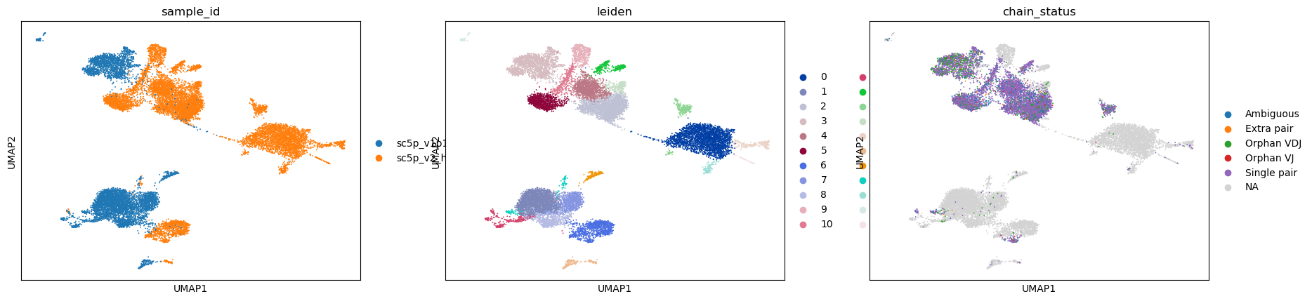
Visualizing the clusters and whether or not there’s a corresponding V(D)J receptor
[18]:
sc.pl.umap(adata, color=["sample_id", "leiden", "chain_status"])
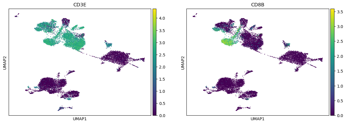
Visualizing some T cell genes
[19]:
sc.pl.umap(adata, color=["CD3E", "CD8B"])
Find clones.
Note
Here we specify identity = 1 so only cells with identical CDR3 nucleotide sequences (key = 'junction') are grouped into clones/clonotypes.
[20]:
ddl.tl.find_clones(vdj, identity=1, key="junction")
vdj
Using PyTorch backend with Apple Metal GPU
Finding clones based on abT cell VDJ chains using junction: 100%|██████████| 2289/2289 [00:07<00:00, 299.18it/s]
Finding clones based on abT cell VJ chains using junction: 100%|██████████| 3754/3754 [00:03<00:00, 992.82it/s]
Building distance matrix (batched): 100%|██████████| 61/61 [00:00<00:00, 747.17it/s]
[20]:
Lazy Dandelion object with n_obs = 6848 and n_contigs = 13343
    data: cell_id, sequence_id, sequence, sequence_aa, productive, rev_comp, v_call, v_cigar, d_call, d_cigar, j_call, j_cigar, c_call, c_cigar, sequence_alignment, germline_alignment, junction, junction_aa, junction_length, junction_aa_length, v_sequence_start, v_sequence_end, d_sequence_start, d_sequence_end, j_sequence_start, j_sequence_end, c_sequence_start, c_sequence_end, consensus_count, umi_count, is_cell, locus, rearrangement_status, extra, ambiguous, clone_id
    metadata: cell_id, clone_id, clone_id_rank, productive_VDJ, productive_VJ, v_call_VDJ, v_call_VJ, d_call_VDJ, j_call_VDJ, j_call_VJ, c_call_VDJ, c_call_VJ, junction_VDJ, junction_VJ, junction_aa_VDJ, junction_aa_VJ, locus_VDJ, locus_VJ, umi_count_VDJ, umi_count_VJ, productive_VDJ_main, productive_VJ_main, v_call_VDJ_main, v_call_VJ_main, d_call_VDJ_main, j_call_VDJ_main, j_call_VJ_main, c_call_VDJ_main, c_call_VJ_main, junction_VDJ_main, junction_VJ_main, junction_aa_VDJ_main, junction_aa_VJ_main, locus_VDJ_main, locus_VJ_main, umi_count_VDJ_main, umi_count_VJ_main, locus_status, chain_status, rearrangement_status_VDJ, rearrangement_status_VJ
    distances: distance matrix of shape (6848, 6848)
Generate TCR network.
The 10x-provided AIRR file is missing columns like sequence_alignment and sequence_alignment_aa so we will use the next best thing, which is sequence or sequence_aa. Note that these columns are not-gapped.
Specify key = 'sequence_aa' to toggle this behavior. Can also try junction or junction_aa if just want to visualise the CDR3 linkage.
[21]:
# again, i'm removing the Orphan VJ cells (lacking TRB chain i.e. VDJ information).
vdj = vdj[
    vdj.metadata.chain_status.is_in(
        ["Single pair", "Extra pair", "Extra pair-exception", "Orphan VDJ"]
    )
].copy()
[22]:
ddl.tl.generate_network(vdj, key="sequence_aa")
[23]:
vdj
[23]:
Lazy Dandelion object with n_obs = 6094 and n_contigs = 11300
    data: cell_id, sequence_id, sequence, sequence_aa, productive, rev_comp, v_call, v_cigar, d_call, d_cigar, j_call, j_cigar, c_call, c_cigar, sequence_alignment, germline_alignment, junction, junction_aa, junction_length, junction_aa_length, v_sequence_start, v_sequence_end, d_sequence_start, d_sequence_end, j_sequence_start, j_sequence_end, c_sequence_start, c_sequence_end, consensus_count, umi_count, is_cell, locus, rearrangement_status, extra, ambiguous, clone_id
    metadata: cell_id, clone_id, clone_id_rank, productive_VDJ, productive_VJ, v_call_VDJ, v_call_VJ, d_call_VDJ, j_call_VDJ, j_call_VJ, c_call_VDJ, c_call_VJ, junction_VDJ, junction_VJ, junction_aa_VDJ, junction_aa_VJ, locus_VDJ, locus_VJ, umi_count_VDJ, umi_count_VJ, productive_VDJ_main, productive_VJ_main, v_call_VDJ_main, v_call_VJ_main, d_call_VDJ_main, j_call_VDJ_main, j_call_VJ_main, c_call_VDJ_main, c_call_VJ_main, junction_VDJ_main, junction_VJ_main, junction_aa_VDJ_main, junction_aa_VJ_main, locus_VDJ_main, locus_VJ_main, umi_count_VDJ_main, umi_count_VJ_main, locus_status, chain_status, rearrangement_status_VDJ, rearrangement_status_VJ
    layout: layout for 6094 vertices, layout for 151 vertices
    graph: networkx graph of 6094 vertices, networkx graph of 151 vertices
    distances: distance matrix of shape (6094, 6094)
Plotting in scanpy.
[24]:
ddl.tl.transfer(adata, vdj)
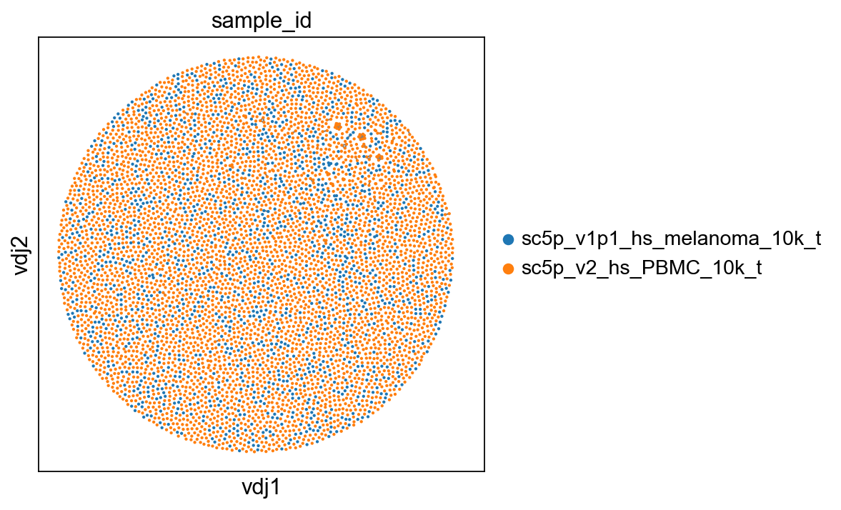
[25]:
sc.set_figure_params(figsize=[5, 5])
ddl.pl.clone_network(adata, color=["sample_id"], edges_width=1, size=15)
[26]:
adata
[26]:
AnnData object with n_obs × n_vars = 17275 × 2305
    obs: 'sample_id', 'n_genes', 'n_genes_by_counts', 'total_counts', 'total_counts_mt', 'pct_counts_mt', 'scrublet_score', 'is_doublet', 'filter_rna', 'has_contig', 'productive_VDJ', 'productive_VJ', 'v_call_VDJ', 'v_call_VJ', 'd_call_VDJ', 'j_call_VDJ', 'j_call_VJ', 'c_call_VDJ', 'c_call_VJ', 'junction_VDJ', 'junction_VJ', 'junction_aa_VDJ', 'junction_aa_VJ', 'locus_VDJ', 'locus_VJ', 'umi_count_VDJ', 'umi_count_VJ', 'productive_VDJ_main', 'productive_VJ_main', 'v_call_VDJ_main', 'v_call_VJ_main', 'd_call_VDJ_main', 'j_call_VDJ_main', 'j_call_VJ_main', 'c_call_VDJ_main', 'c_call_VJ_main', 'junction_VDJ_main', 'junction_VJ_main', 'junction_aa_VDJ_main', 'junction_aa_VJ_main', 'locus_VDJ_main', 'locus_VJ_main', 'umi_count_VDJ_main', 'umi_count_VJ_main', 'locus_status', 'chain_status', 'rearrangement_status_VDJ', 'rearrangement_status_VJ', 'leiden', 'clone_id', 'clone_id_rank'
    var: 'n_cells', 'highly_variable', 'means', 'dispersions', 'dispersions_norm', 'mean', 'std'
    uns: 'log1p', 'hvg', 'pca', 'neighbors', 'umap', 'leiden', 'sample_id_colors', 'leiden_colors', 'chain_status_colors', 'dandelion', 'gex_neighbors', 'clone_id'
    obsm: 'X_pca', 'X_umap', 'X_vdj'
    varm: 'PCs'
    obsp: 'distances', 'connectivities'
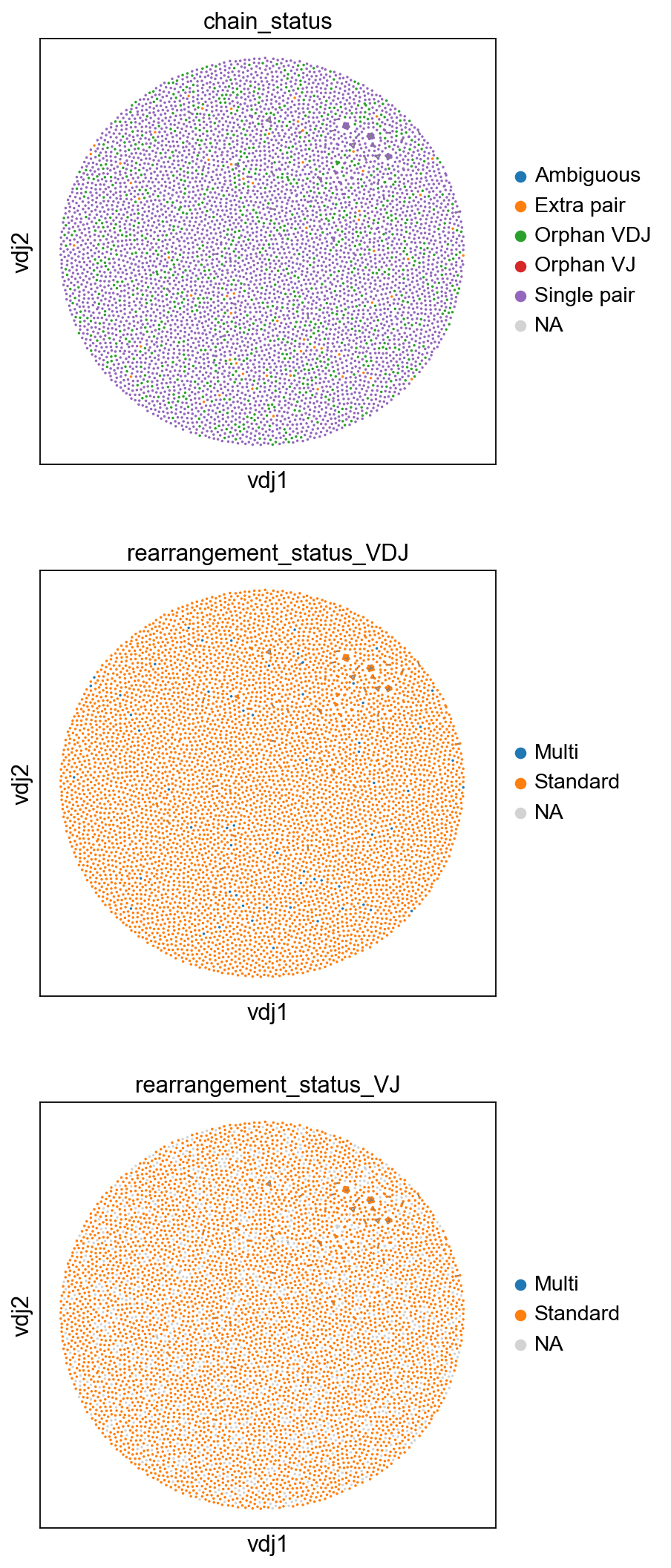
[27]:
sc.set_figure_params(figsize=[4.5, 5])
ddl.pl.clone_network(
    adata,
    color=[
        "chain_status",
        "rearrangement_status_VDJ",
        "rearrangement_status_VJ",
    ],
    ncols=1,
    legend_fontoutline=3,
    size=10,
    edges_width=1,
)
[28]:
ddl.tl.transfer(adata, vdj)
adata
[28]:
AnnData object with n_obs × n_vars = 17275 × 2305
    obs: 'sample_id', 'n_genes', 'n_genes_by_counts', 'total_counts', 'total_counts_mt', 'pct_counts_mt', 'scrublet_score', 'is_doublet', 'filter_rna', 'has_contig', 'productive_VDJ', 'productive_VJ', 'v_call_VDJ', 'v_call_VJ', 'd_call_VDJ', 'j_call_VDJ', 'j_call_VJ', 'c_call_VDJ', 'c_call_VJ', 'junction_VDJ', 'junction_VJ', 'junction_aa_VDJ', 'junction_aa_VJ', 'locus_VDJ', 'locus_VJ', 'umi_count_VDJ', 'umi_count_VJ', 'productive_VDJ_main', 'productive_VJ_main', 'v_call_VDJ_main', 'v_call_VJ_main', 'd_call_VDJ_main', 'j_call_VDJ_main', 'j_call_VJ_main', 'c_call_VDJ_main', 'c_call_VJ_main', 'junction_VDJ_main', 'junction_VJ_main', 'junction_aa_VDJ_main', 'junction_aa_VJ_main', 'locus_VDJ_main', 'locus_VJ_main', 'umi_count_VDJ_main', 'umi_count_VJ_main', 'locus_status', 'chain_status', 'rearrangement_status_VDJ', 'rearrangement_status_VJ', 'leiden', 'clone_id', 'clone_id_rank'
    var: 'n_cells', 'highly_variable', 'means', 'dispersions', 'dispersions_norm', 'mean', 'std'
    uns: 'log1p', 'hvg', 'pca', 'neighbors', 'umap', 'leiden', 'sample_id_colors', 'leiden_colors', 'chain_status_colors', 'dandelion', 'gex_neighbors', 'clone_id', 'rearrangement_status_VDJ_colors', 'rearrangement_status_VJ_colors'
    obsm: 'X_pca', 'X_umap', 'X_vdj'
    varm: 'PCs'
    obsp: 'distances', 'connectivities'
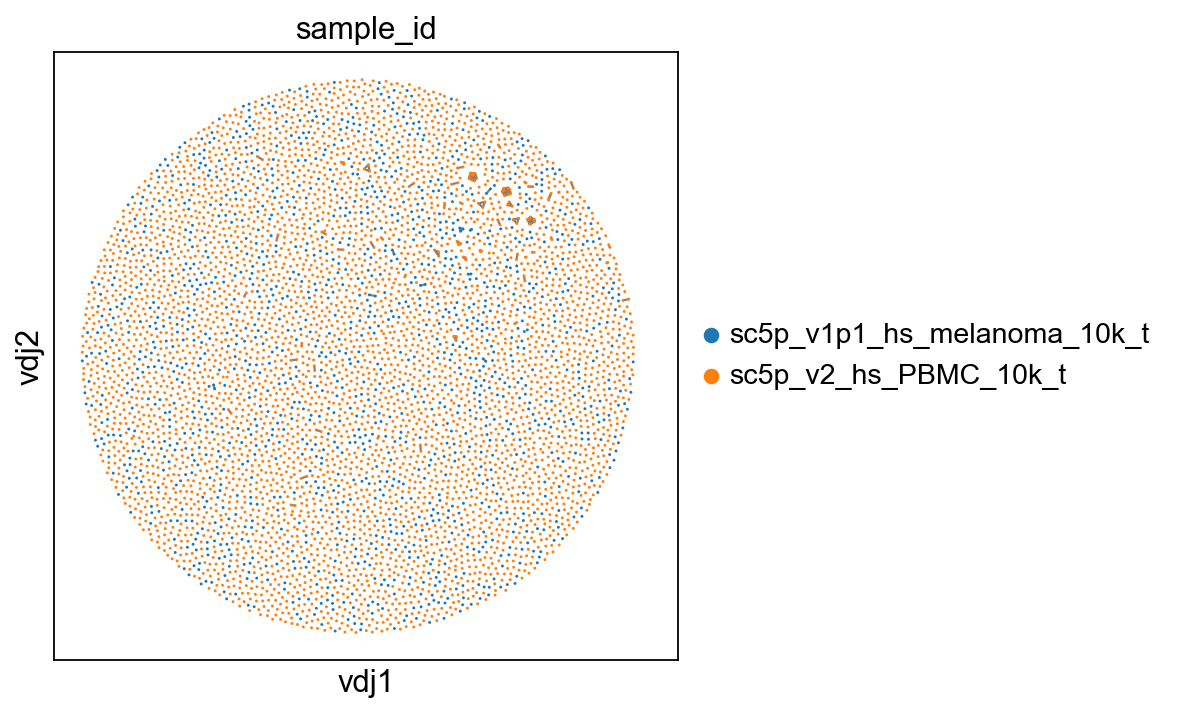
[29]:
sc.set_figure_params(figsize=[5, 5])
ddl.pl.clone_network(adata, color=["sample_id"], edges_width=1)
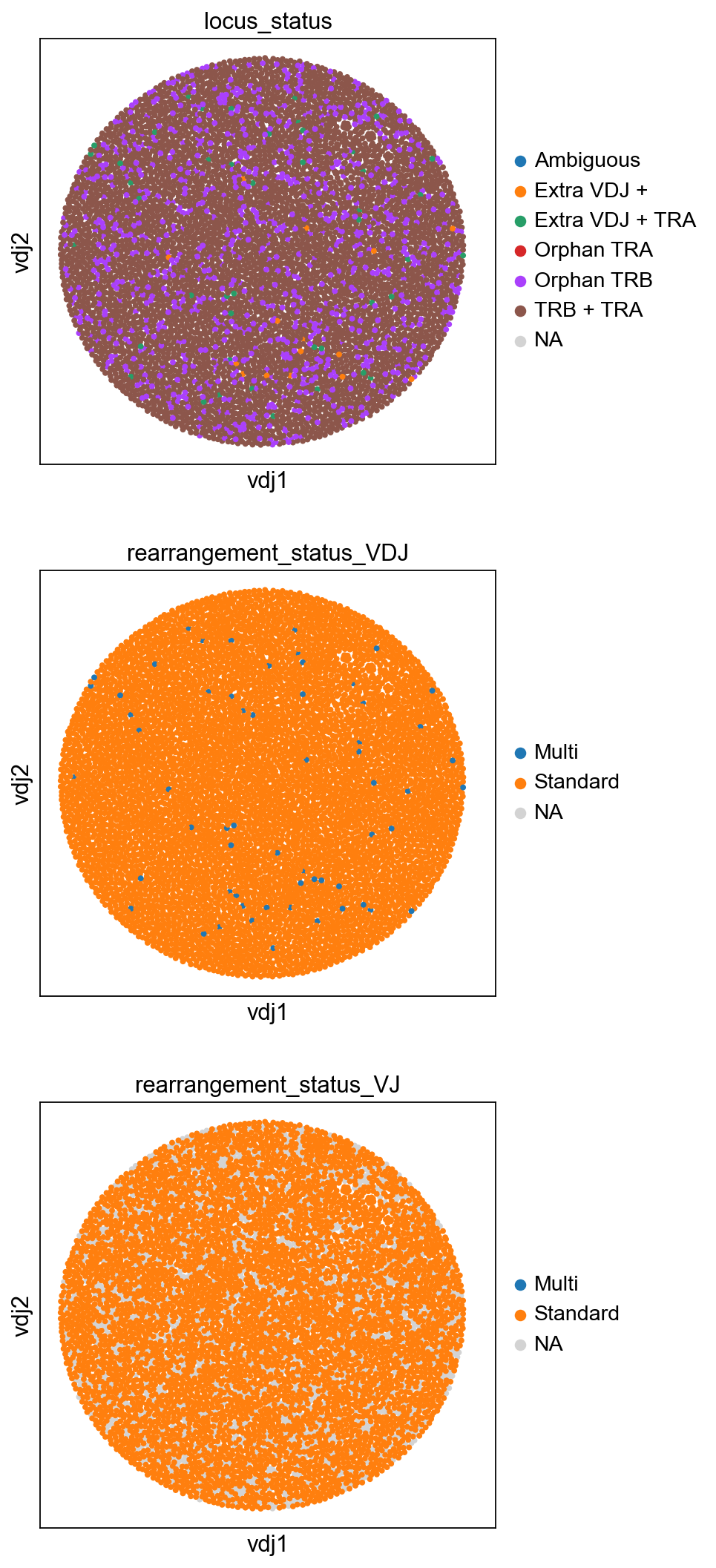
[30]:
sc.set_figure_params(figsize=[4.5, 5])
ddl.pl.clone_network(
    adata,
    color=[
        "locus_status",
        "rearrangement_status_VDJ",
        "rearrangement_status_VJ",
    ],
    ncols=1,
    legend_fontoutline=3,
    edges_width=1,
    size=50,
)
Using scirpy to plot
You can also use scirpy’s functions to plot the network.
A likely use case is if you have a lot of cells and you don’t want to wait for dandelion to generate the layout because it’s taking too long. Or you simply prefer scirpy’s style of plotting.
You can run ddl.tl.generate_network(..., compute_graph = False) and it will skip the graph construction and layout computation, and after transfer to scirpy, you can use its plotting functions to visualise the networks - the clone network is generated very quickly but visualising it using spring layout does take quite a while.
To access scirpy’s functions, you would first need to do a Dandelion to scirpy conversion first with ddl.to_scirpy(...).
[31]:
import scirpy as ir

iradata = ddl.tl.to_scirpy(vdj, gex_adata=adata, transfer=True)
iradata
[31]:
MuData object with n_obs × n_vars = 17275 × 2305
2 modalities
gex: 17275 x 2305
obs: 'sample_id', 'n_genes', 'n_genes_by_counts', 'total_counts', 'total_counts_mt', 'pct_counts_mt', 'scrublet_score', 'is_doublet', 'filter_rna', 'has_contig', 'productive_VDJ', 'productive_VJ', 'v_call_VDJ', 'v_call_VJ', 'd_call_VDJ', 'j_call_VDJ', 'j_call_VJ', 'c_call_VDJ', 'c_call_VJ', 'junction_VDJ', 'junction_VJ', 'junction_aa_VDJ', 'junction_aa_VJ', 'locus_VDJ', 'locus_VJ', 'umi_count_VDJ', 'umi_count_VJ', 'productive_VDJ_main', 'productive_VJ_main', 'v_call_VDJ_main', 'v_call_VJ_main', 'd_call_VDJ_main', 'j_call_VDJ_main', 'j_call_VJ_main', 'c_call_VDJ_main', 'c_call_VJ_main', 'junction_VDJ_main', 'junction_VJ_main', 'junction_aa_VDJ_main', 'junction_aa_VJ_main', 'locus_VDJ_main', 'locus_VJ_main', 'umi_count_VDJ_main', 'umi_count_VJ_main', 'locus_status', 'chain_status', 'rearrangement_status_VDJ', 'rearrangement_status_VJ', 'leiden', 'clone_id', 'clone_id_rank'
var: 'n_cells', 'highly_variable', 'means', 'dispersions', 'dispersions_norm', 'mean', 'std'
uns: 'log1p', 'hvg', 'pca', 'neighbors', 'umap', 'leiden', 'sample_id_colors', 'leiden_colors', 'chain_status_colors', 'dandelion', 'gex_neighbors', 'clone_id', 'rearrangement_status_VDJ_colors', 'rearrangement_status_VJ_colors', 'locus_status_colors'
obsm: 'X_pca', 'X_umap', 'X_vdj'
varm: 'PCs'
obsp: 'distances', 'connectivities'
airr: 6094 x 0
obs: 'clone_id', 'clone_id_rank', 'productive_VDJ', 'productive_VJ', 'v_call_VDJ', 'v_call_VJ', 'd_call_VDJ', 'j_call_VDJ', 'j_call_VJ', 'c_call_VDJ', 'c_call_VJ', 'junction_VDJ', 'junction_VJ', 'junction_aa_VDJ', 'junction_aa_VJ', 'locus_VDJ', 'locus_VJ', 'umi_count_VDJ', 'umi_count_VJ', 'productive_VDJ_main', 'productive_VJ_main', 'v_call_VDJ_main', 'v_call_VJ_main', 'd_call_VDJ_main', 'j_call_VDJ_main', 'j_call_VJ_main', 'c_call_VDJ_main', 'c_call_VJ_main', 'junction_VDJ_main', 'junction_VJ_main', 'junction_aa_VDJ_main', 'junction_aa_VJ_main', 'locus_VDJ_main', 'locus_VJ_main', 'umi_count_VDJ_main', 'umi_count_VJ_main', 'locus_status', 'chain_status', 'rearrangement_status_VDJ', 'rearrangement_status_VJ'
uns: 'clone_id', 'dandelion', 'neighbors'
obsm: 'airr', 'X_vdj'
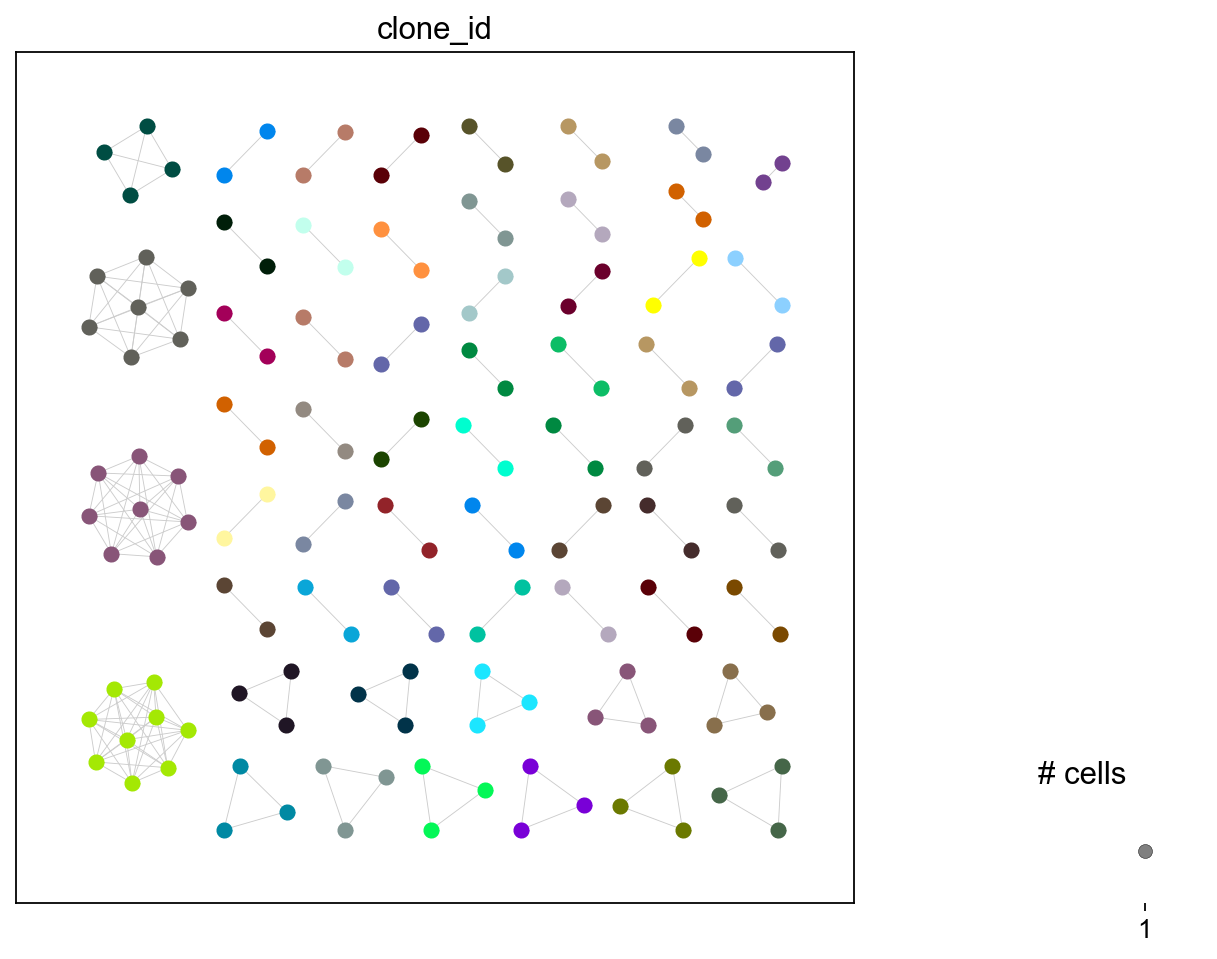
obsp: 'connectivities', 'distances'[32]:
ir.tl.clonotype_network(iradata, min_cells=2)
ir.pl.clonotype_network(
    iradata, color="clone_id", panel_size=(7, 7), show_labels=False
)
[32]:
<Axes: >
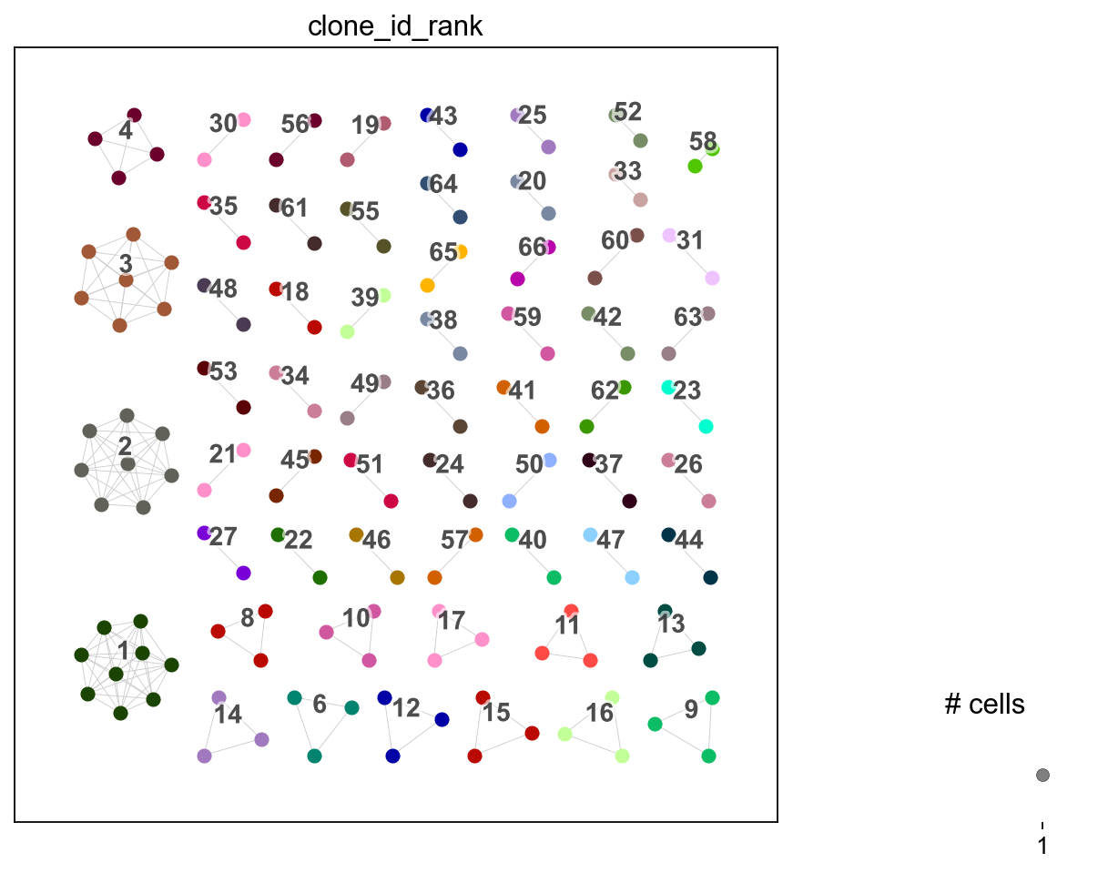
You can change the clonotype labels by transferring with a different clone_key. For example, using clone_id_rank which is numerically ordered from largest to smallest in ascending order where 1 is the largest clone and so on.
[33]:
ddl.tl.transfer(iradata, vdj, clone_key="clone_id_rank")
ir.tl.clonotype_network(iradata, clonotype_key="clone_id_rank", min_cells=2)
ir.pl.clonotype_network(iradata, color="clone_id_rank", panel_size=(7, 7))
[33]:
<Axes: >
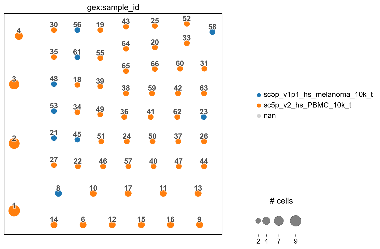
You can also transfer with the clones collapsed for plotting as pie-charts as per how scirpy does it.
[34]:
ddl.tl.transfer(iradata, vdj, clone_key="clone_id_rank", collapse_nodes=True)
ir.tl.clonotype_network(iradata, clonotype_key="clone_id_rank", min_cells=2)
ir.pl.clonotype_network(iradata, color="gex:sample_id", panel_size=(7, 7))
[34]:
<Axes: >
Finish.
We can save the files.
[35]:
adata.write("adata_tcr.h5ad", compression="gzip")
[38]:
vdj.write_zipddl("dandelion_results_tcr.zipddl")