V(D)J clustering
On the topic of finding clones/clonotypes, there are many ways used for clustering BCRs, almost all involving some measure based on sequence similarity. There are also a lot of very well established guidelines and criterias maintained by the BCR community. For example, immcantation uses a number of model-based methods that performs clustering of amino acid or nucleotide sequences based on predetermined thresholds (either user-selected or using a density-based approach).
Here, dandelion implements a convenient method to call clones using a simple nearest-neighbor approach that satisfies the criteria described below. But first, let’s load the modules and files we need.
[1]:
import os
import scanpy as sc
import dandelion as ddl

os.chdir("dandelion_tutorial")
sc.settings.verbosity = 3
[2]:
# read in the previously saved file
vdj = ddl.read_zipddl("dandelion_results.zipddl")
vdj
[2]:
Lazy Dandelion object with n_obs = 2496 and n_contigs = 5792
    data: sequence_id, sequence, rev_comp, productive, v_call, d_call, j_call, sequence_alignment, germline_alignment, junction, junction_aa, v_cigar, d_cigar, j_cigar, stop_codon, vj_in_frame, locus, junction_length, np1_length, np2_length, v_sequence_start, v_sequence_end, v_germline_start, v_germline_end, d_sequence_start, d_sequence_end, d_germline_start, d_germline_end, j_sequence_start, j_sequence_end, j_germline_start, j_germline_end, v_score, v_identity, v_support, d_score, d_identity, d_support, j_score, j_identity, j_support, fwr1, fwr2, fwr3, fwr4, cdr1, cdr2, cdr3, cell_id, consensus_count, umi_count, v_call_10x, d_call_10x, j_call_10x, junction_10x, junction_10x_aa, j_call_blastn, j_identity_blastn, j_alignment_length_blastn, j_number_of_mismatches_blastn, j_number_of_gap_openings_blastn, j_sequence_start_blastn, j_sequence_end_blastn, j_germline_start_blastn, j_germline_end_blastn, j_support_blastn, j_score_blastn, j_sequence_alignment_blastn, j_germline_alignment_blastn, j_call_igblastn, j_source, j_support_igblastn, j_score_igblastn, d_call_blastn, d_identity_blastn, d_alignment_length_blastn, d_number_of_mismatches_blastn, d_number_of_gap_openings_blastn, d_sequence_start_blastn, d_sequence_end_blastn, d_germline_start_blastn, d_germline_end_blastn, d_support_blastn, d_score_blastn, d_sequence_alignment_blastn, d_germline_alignment_blastn, d_call_igblastn, d_source, d_support_igblastn, d_score_igblastn, v_call_genotyped, germline_alignment_d_mask, sample_id, c_call, c_sequence_alignment, c_germline_alignment, c_sequence_start, c_sequence_end, c_score, c_identity, c_call_10x, junction_aa_length, fwr1_aa, fwr2_aa, fwr3_aa, fwr4_aa, cdr1_aa, cdr2_aa, cdr3_aa, sequence_alignment_aa, v_sequence_alignment_aa, d_sequence_alignment_aa, j_sequence_alignment_aa, complete_vdj, j_call_multimappers, j_call_multiplicity, j_call_sequence_start_multimappers, j_call_sequence_end_multimappers, j_call_support_multimappers, mu_count, rearrangement_status, v_call_functionality, d_call_functionality, j_call_functionality, extra, ambiguous
    metadata: cell_id, sample_id, productive_VDJ, productive_VJ, d_call_VDJ, j_call_VDJ, j_call_VJ, junction_VDJ, junction_VJ, junction_aa_VDJ, junction_aa_VJ, locus_VDJ, locus_VJ, v_call_VDJ, v_call_VJ, c_call_VDJ, c_call_VJ, umi_count_VDJ, umi_count_VJ, productive_VDJ_main, productive_VJ_main, d_call_VDJ_main, j_call_VDJ_main, j_call_VJ_main, junction_VDJ_main, junction_VJ_main, junction_aa_VDJ_main, junction_aa_VJ_main, locus_VDJ_main, locus_VJ_main, v_call_genotyped_VDJ_main, v_call_genotyped_VJ_main, c_call_VDJ_main, c_call_VJ_main, umi_count_VDJ_main, umi_count_VJ_main, isotype, isotype_main, isotype_status, locus_status, chain_status, rearrangement_status_VDJ, rearrangement_status_VJ
[3]:
adata = sc.read_h5ad("adata.h5ad")
adata
[3]:
AnnData object with n_obs × n_vars = 25063 × 1309
    obs: 'sample_id', 'n_genes', 'n_genes_by_counts', 'total_counts', 'total_counts_mt', 'pct_counts_mt', 'gmm_pct_count_clusters_keep', 'scrublet_score', 'is_doublet', 'filter_rna', 'has_contig', 'productive_VDJ', 'productive_VJ', 'd_call_VDJ', 'j_call_VDJ', 'j_call_VJ', 'junction_VDJ', 'junction_VJ', 'junction_aa_VDJ', 'junction_aa_VJ', 'locus_VDJ', 'locus_VJ', 'v_call_VDJ', 'v_call_VJ', 'c_call_VDJ', 'c_call_VJ', 'umi_count_VDJ', 'umi_count_VJ', 'productive_VDJ_main', 'productive_VJ_main', 'd_call_VDJ_main', 'j_call_VDJ_main', 'j_call_VJ_main', 'junction_VDJ_main', 'junction_VJ_main', 'junction_aa_VDJ_main', 'junction_aa_VJ_main', 'locus_VDJ_main', 'locus_VJ_main', 'v_call_genotyped_VDJ_main', 'v_call_genotyped_VJ_main', 'c_call_VDJ_main', 'c_call_VJ_main', 'umi_count_VDJ_main', 'umi_count_VJ_main', 'isotype', 'isotype_main', 'isotype_status', 'locus_status', 'chain_status', 'rearrangement_status_VDJ', 'rearrangement_status_VJ', 'leiden'
    var: 'n_cells', 'highly_variable', 'means', 'dispersions', 'dispersions_norm', 'mean', 'std'
    uns: 'chain_status_colors', 'hvg', 'leiden', 'leiden_colors', 'log1p', 'neighbors', 'pca', 'sample_id_colors', 'umap'
    obsm: 'X_pca', 'X_umap'
    varm: 'PCs'
    obsp: 'connectivities', 'distances'
Finding clones
The following is dandelion’s implementation of a rather conventional method to define clones, ddl.tl.find_clones.
Clone definition criterion
Clone definition is based on the following criterion:
Identical V- and J-gene usage in the VDJ chain (IGH/TRB/TRD).
Identical CDR3 junctional/CDR3 sequence length in the VDJ chain.
VDJ chain junctional/CDR3 sequences attains a minimum of % sequence similarity, based on hamming distance. The similarity cut-off is tunable (default is 85%; change to 100% if analyzing TCR data).
VJ chain (IGK/IGL/TRA/TRG) usage. If cells within clones use different VJ chains, the clone will be split following the same conditions for VDJ chains in (1-3) as above.
(Optional) Simplifying annotation calls.
This is an optional step to simplify the annotation calls. The vdj.simplify() will reduce the complexity of the gene names and strip the alleles. This impacts on how clones are defined (using simpler v/j calls) and also visualiation.
[4]:
# original
vdj.data[["v_call_genotyped", "j_call", "c_call"]].collect()
[4]:
| v_call_genotyped | j_call | c_call |
|---|---|---|
| str | str | str |
| "IGKV1-33*01,IGKV1D-33*01" | "IGKJ4*01" | "IGKC" |
| "IGHV1-69*01,IGHV1-69D*01" | "IGHJ3*02" | "IGHM" |
| "IGKV1-8*01" | "IGKJ1*01" | "IGKC" |
| "IGLV5-45*02" | "IGLJ3*02" | "IGLC3" |
| "IGHV1-2*02" | "IGHJ3*02" | "IGHM" |
| … | … | … |
| "IGHV1-46*01" | "IGHJ5*02" | "IGHM" |
| "IGHV1-69*01,IGHV1-69D*01" | "IGHJ6*02" | "IGHM" |
| "IGLV1-47*01" | "IGLJ3*02" | "IGLC3" |
| "IGLV2-11*01" | "IGLJ2*01,IGLJ3*01,IGLJ3*02" | "IGLC" |
| "IGHV3-23*01,IGHV3-23D*01" | "IGHJ4*02" | "IGHM" |
[5]:
vdj.simplify()
vdj.data[["v_call_genotyped", "j_call", "c_call"]].collect()
[5]:
| v_call_genotyped | j_call | c_call |
|---|---|---|
| str | str | str |
| "IGKV1-33" | "IGKJ4" | "IGKC" |
| "IGHV1-69" | "IGHJ3" | "IGHM" |
| "IGKV1-8" | "IGKJ1" | "IGKC" |
| "IGLV5-45" | "IGLJ3" | "IGLC3" |
| "IGHV1-2" | "IGHJ3" | "IGHM" |
| … | … | … |
| "IGHV1-46" | "IGHJ5" | "IGHM" |
| "IGHV1-69" | "IGHJ6" | "IGHM" |
| "IGLV1-47" | "IGLJ3" | "IGLC3" |
| "IGLV2-11" | "IGLJ2" | "IGLC" |
| "IGHV3-23" | "IGHJ4" | "IGHM" |
[6]:
# let's save this as a separate file
vdj.write_zipddl("dandelion_results_simplified.zipddl")
Running ddl.tl.find_clones
The function will take a file path, a polars DataFrame (for example if you’ve used polars to read in the filtered file already), or a DandelionPolars class object. The default mode for calculation of junctional hamming distance is to use the CDR3 junction amino acid sequences, specified via the key option (None defaults to junction_aa). You can switch it to using CDR3 junction nucleotide sequences by specifying key='junction'.
store_distances=True
Setting store_distances=True will store the clone-level pairwise distance matrix as a CSR sparse matrix in vdj.distances. This is useful because ddl.tl.generate_network will automatically detect and reuse pre-computed distances from .distances, avoiding redundant recalculation. This can save significant time when running both find_clones and generate_network in sequence.
[7]:
ddl.tl.find_clones(vdj, store_distances=True)
vdj.distances
Finding clonotypes
Using PyTorch backend with Apple Metal GPU
Finding clones based on B cell VDJ chains using junction_aa: 100%|██████████| 1177/1177 [00:01<00:00, 799.66it/s]
Finding clones based on B cell VJ chains using junction_aa: 100%|██████████| 492/492 [00:00<00:00, 794.81it/s]
Storing distance matrix...
Building distance matrix (batched): 100%|██████████| 17/17 [00:00<00:00, 3271.09it/s]
Stored distances as CSR sparse matrix: (2496, 2496), density=0.69%
 finished: Updated Dandelion object:
   'data', contig AIRR table
   'metadata', cell observations table
   'distances', sparse distance matrix
 (0:00:03)
[7]:
<Compressed Sparse Row sparse matrix of dtype 'float32'
        with 42933 stored elements and shape (2496, 2496)>
This will return a new column with the column name 'clone_id' as per convention. If a file path is provided as input, it will also save the file automatically into the base directory of the file name. Otherwise, a DandelionPolars object will be returned.
Clonotype definition criterion
The clone_id follows an VDJ_{A}_{B}_{C}_VJ_{D}_{E}_{F} format and largely reflects the conditions above where:
{A} indicates if the contigs use the same V and J genes in the VDJ chain.

{B} indicates if junctional/CDR3 sequences are equal in length in the VDJ chain.

{C} indicates if clones are split based on distance threshold for the VDJ chain.

{D} indicates if the contigs use the same V and J genes in the VJ chain.

{E} indicates if junctional/CDR3 sequences are equal in length in the VJ chain.

{F} indicates if clones are split based on distance threshold for the VJ chain.
[8]:
vdj.metadata.collect()
[8]:
| cell_id | clone_id | clone_id_rank | sample_id | productive_VDJ | productive_VJ | d_call_VDJ | j_call_VDJ | j_call_VJ | junction_VDJ | junction_VJ | junction_aa_VDJ | junction_aa_VJ | locus_VDJ | locus_VJ | v_call_VDJ | v_call_VJ | c_call_VDJ | c_call_VJ | umi_count_VDJ | umi_count_VJ | productive_VDJ_main | productive_VJ_main | d_call_VDJ_main | j_call_VDJ_main | j_call_VJ_main | junction_VDJ_main | junction_VJ_main | junction_aa_VDJ_main | junction_aa_VJ_main | locus_VDJ_main | locus_VJ_main | v_call_genotyped_VDJ_main | v_call_genotyped_VJ_main | c_call_VDJ_main | c_call_VJ_main | umi_count_VDJ_main | umi_count_VJ_main | isotype | isotype_main | isotype_status | locus_status | chain_status | rearrangement_status_VDJ | rearrangement_status_VJ |
|---|---|---|---|---|---|---|---|---|---|---|---|---|---|---|---|---|---|---|---|---|---|---|---|---|---|---|---|---|---|---|---|---|---|---|---|---|---|---|---|---|---|---|---|---|
| str | str | cat | str | str | str | str | str | str | str | str | str | str | str | str | str | str | str | str | i64 | i64 | str | str | str | str | str | str | str | str | str | str | str | str | str | str | str | f64 | f64 | str | str | str | str | str | str | str |
| "sc5p_v2_hs_PBMC_10k_b_AAACCTGT… | "B_VJ_22_2_2" | "2384" | "sc5p_v2_hs_PBMC_10k_b" | null | "T" | null | null | "IGKJ4" | null | "TGTCAACAATATGACGAACTTCCCGTCACT… | null | "CQQYDELPVTF" | null | "IGK" | null | "IGKV1-33" | null | "IGKC" | 0 | 68 | null | "T" | null | null | "IGKJ4" | null | "TGTCAACAATATGACGAACTTCCCGTCACT… | null | "CQQYDELPVTF" | null | "IGK" | null | "IGKV1-33" | null | "IGKC" | null | 68.0 | null | null | null | "Orphan IGK" | "Orphan VJ" | null | "Standard" |
| "sc5p_v2_hs_PBMC_10k_b_AAACCTGT… | "B_VDJ_32_4_1_VJ_39_2_1" | "921" | "sc5p_v2_hs_PBMC_10k_b" | "T" | "T" | "IGHD3-22" | "IGHJ3" | "IGKJ1" | "TGTGCGACTACGTATTACTATGATAGTAGT… | "TGTCAACAGTATTATAGTTACCCTCGGACG… | "CATTYYYDSSGYYQNDAFDIW" | "CQQYYSYPRTF" | "IGH" | "IGK" | "IGHV1-69" | "IGKV1-8" | "IGHM" | "IGKC" | 51 | 43 | "T" | "T" | "IGHD3-22" | "IGHJ3" | "IGKJ1" | "TGTGCGACTACGTATTACTATGATAGTAGT… | "TGTCAACAGTATTATAGTTACCCTCGGACG… | "CATTYYYDSSGYYQNDAFDIW" | "CQQYYSYPRTF" | "IGH" | "IGK" | "IGHV1-69" | "IGKV1-8" | "IGHM" | "IGKC" | 51.0 | 43.0 | "IgM" | "IgM" | "IgM" | "IGH + IGK" | "Single pair" | "Standard" | "Standard" |
| "sc5p_v2_hs_PBMC_10k_b_AAACCTGT… | "B_VDJ_8_1_2_VJ_190_1_1" | "941" | "sc5p_v2_hs_PBMC_10k_b" | "T" | "T" | null | "IGHJ3" | "IGLJ3" | "TGTGCGAGAGAGATAGAGGGGGACGGTGTT… | "TGTATGATTTGGCACAGCAGCGCTTGGGTG… | "CAREIEGDGVFEIW" | "CMIWHSSAWVV" | "IGH" | "IGL" | "IGHV1-2" | "IGLV5-45" | "IGHM" | "IGLC3" | 47 | 90 | "T" | "T" | null | "IGHJ3" | "IGLJ3" | "TGTGCGAGAGAGATAGAGGGGGACGGTGTT… | "TGTATGATTTGGCACAGCAGCGCTTGGGTG… | "CAREIEGDGVFEIW" | "CMIWHSSAWVV" | "IGH" | "IGL" | "IGHV1-2" | "IGLV5-45" | "IGHM" | "IGLC3" | 47.0 | 90.0 | "IgM" | "IgM" | "IgM" | "IGH + IGL" | "Single pair" | "Standard" | "Standard" |
| "sc5p_v2_hs_PBMC_10k_b_AAACCTGT… | "B_VDJ_204_4_3_VJ_60_1_1" | "1184" | "sc5p_v2_hs_PBMC_10k_b" | "T" | "T" | null | "IGHJ3" | "IGKJ2" | "TGTGCGAGACATATCCGTGGGAACAGATTT… | "TGTCAACAGTATTATAGTTTCCCGTACACT… | "CARHIRGNRFGNDAFDIW" | "CQQYYSFPYTF" | "IGH" | "IGK" | "IGHV5-51" | "IGKV1D-8" | "IGHM" | "IGKC" | 80 | 22 | "T" | "T" | null | "IGHJ3" | "IGKJ2" | "TGTGCGAGACATATCCGTGGGAACAGATTT… | "TGTCAACAGTATTATAGTTTCCCGTACACT… | "CARHIRGNRFGNDAFDIW" | "CQQYYSFPYTF" | "IGH" | "IGK" | "IGHV5-51" | "IGKV1D-8" | "IGHM" | "IGKC" | 80.0 | 22.0 | "IgM" | "IgM" | "IgM" | "IGH + IGK" | "Single pair" | "Standard" | "Standard" |
| "sc5p_v2_hs_PBMC_10k_b_AAACGGGA… | "B_VDJ_182_2_1_VJ_164_2_1" | "1697" | "sc5p_v2_hs_PBMC_10k_b" | "T" | "T" | "IGHD6-13" | "IGHJ3" | "IGLJ2" | "TGTGCGAGAGTAGGCTATAGAGCAGCAGCT… | "TGTAACTCCCGGGACAGCAGTGGTAACCAT… | "CARVGYRAAAGTDAFDIW" | "CNSRDSSGNHVVF" | "IGH" | "IGL" | "IGHV4-4" | "IGLV3-19" | "IGHM" | "IGLC" | 18 | 14 | "T" | "T" | "IGHD6-13" | "IGHJ3" | "IGLJ2" | "TGTGCGAGAGTAGGCTATAGAGCAGCAGCT… | "TGTAACTCCCGGGACAGCAGTGGTAACCAT… | "CARVGYRAAAGTDAFDIW" | "CNSRDSSGNHVVF" | "IGH" | "IGL" | "IGHV4-4" | "IGLV3-19" | "IGHM" | "IGLC" | 18.0 | 14.0 | "IgM" | "IgM" | "IgM" | "IGH + IGL" | "Single pair" | "Standard" | "Standard" |
| … | … | … | … | … | … | … | … | … | … | … | … | … | … | … | … | … | … | … | … | … | … | … | … | … | … | … | … | … | … | … | … | … | … | … | … | … | … | … | … | … | … | … | … | … |
| "vdj_v1_hs_pbmc3_b_TTTCCTCAGCGC… | "B_VDJ_90_5_2_VJ_73_1_1" | "819" | "vdj_v1_hs_pbmc3_b" | "T" | "T" | "IGHD4-17" | "IGHJ6" | "IGKJ2" | "TGTGCGAAAGCCGCCTACGGTGAGGGGCTC… | "TGCATGCAAGGTACACACTGGCCGTACACT… | "CAKAAYGEGLRYYYYGMDVW" | "CMQGTHWPYTF" | "IGH" | "IGK" | "IGHV3-30" | "IGKV2-30" | "IGHM" | "IGKC" | 11 | 28 | "T" | "T" | "IGHD4-17" | "IGHJ6" | "IGKJ2" | "TGTGCGAAAGCCGCCTACGGTGAGGGGCTC… | "TGCATGCAAGGTACACACTGGCCGTACACT… | "CAKAAYGEGLRYYYYGMDVW" | "CMQGTHWPYTF" | "IGH" | "IGK" | "IGHV3-30" | "IGKV2-30" | "IGHM" | "IGKC" | 11.0 | 28.0 | "IgM" | "IgM" | "IgM" | "IGH + IGK" | "Single pair" | "Standard" | "Standard" |
| "vdj_v1_hs_pbmc3_b_TTTCCTCAGGGA… | "B_VDJ_193_2_1_VJ_25_4_1" | "2073" | "vdj_v1_hs_pbmc3_b" | "T" | "T" | "IGHD6-13" | "IGHJ2" | "IGKJ1" | "TGTGCGAGACCCCGTATAGCAGGATCTGGG… | "TGTCAACAGAGTTACAGTACCCCGTGGACG… | "CARPRIAGSGWYFDLW" | "CQQSYSTPWTF" | "IGH" | "IGK" | "IGHV4-61" | "IGKV1-39" | "IGHM" | "IGKC" | 14 | 159 | "T" | "T" | "IGHD6-13" | "IGHJ2" | "IGKJ1" | "TGTGCGAGACCCCGTATAGCAGGATCTGGG… | "TGTCAACAGAGTTACAGTACCCCGTGGACG… | "CARPRIAGSGWYFDLW" | "CQQSYSTPWTF" | "IGH" | "IGK" | "IGHV4-61" | "IGKV1-39" | "IGHM" | "IGKC" | 14.0 | 159.0 | "IgM" | "IgM" | "IgM" | "IGH + IGK" | "Single pair" | "Standard" | "Standard" |
| "vdj_v1_hs_pbmc3_b_TTTCCTCTCGAC… | "B_VDJ_27_5_2_VJ_26_2_1" | "633" | "vdj_v1_hs_pbmc3_b" | "T" | "T" | "IGHD2-15" | "IGHJ5" | "IGKJ2" | "TGTGCGAGAGAGGGATATTGTAGTGGTGGT… | "TGTCAACAGAGTTACAGTACCCCTCGGACT… | "CAREGYCSGGSCYSPDPNNGWFDPW" | "CQQSYSTPRTF" | "IGH" | "IGK" | "IGHV1-46" | "IGKV1-39" | "IGHM" | "IGKC" | 28 | 35 | "T" | "T" | "IGHD2-15" | "IGHJ5" | "IGKJ2" | "TGTGCGAGAGAGGGATATTGTAGTGGTGGT… | "TGTCAACAGAGTTACAGTACCCCTCGGACT… | "CAREGYCSGGSCYSPDPNNGWFDPW" | "CQQSYSTPRTF" | "IGH" | "IGK" | "IGHV1-46" | "IGKV1-39" | "IGHM" | "IGKC" | 28.0 | 35.0 | "IgM" | "IgM" | "IgM" | "IGH + IGK" | "Single pair" | "Standard" | "Standard" |
| "vdj_v1_hs_pbmc3_b_TTTGCGCCATAC… | "B_VDJ_35_7_2_VJ_134_3_1" | "1027" | "vdj_v1_hs_pbmc3_b" | "T" | "T" | "IGHD2-15" | "IGHJ6" | "IGLJ3" | "TGTGCGAGATCTCTGGATATTGTAGTGGTG… | "TGTGCAGCATGGGATGACAGCCTGAGTGGT… | "CARSLDIVVVVALYYYYGMDVW" | "CAAWDDSLSGWVF" | "IGH" | "IGL" | "IGHV1-69" | "IGLV1-47" | "IGHM" | "IGLC3" | 32 | 28 | "T" | "T" | "IGHD2-15" | "IGHJ6" | "IGLJ3" | "TGTGCGAGATCTCTGGATATTGTAGTGGTG… | "TGTGCAGCATGGGATGACAGCCTGAGTGGT… | "CARSLDIVVVVALYYYYGMDVW" | "CAAWDDSLSGWVF" | "IGH" | "IGL" | "IGHV1-69" | "IGLV1-47" | "IGHM" | "IGLC3" | 32.0 | 28.0 | "IgM" | "IgM" | "IgM" | "IGH + IGL" | "Single pair" | "Standard" | "Standard" |
| "vdj_v1_hs_pbmc3_b_TTTGGTTGTAGG… | "B_VDJ_82_6_1_VJ_141_3_1" | "694" | "vdj_v1_hs_pbmc3_b" | "T" | "T" | null | "IGHJ4" | "IGLJ2" | "TGTGCGGGGAGTCGGTGGTTATATTCTTTT… | "TGCTGCTCATATGCAGGCAGCTACACTGTG… | "CAGSRWLYSFDYW" | "CCSYAGSYTVFF" | "IGH" | "IGL" | "IGHV3-23" | "IGLV2-11" | "IGHM" | "IGLC" | 22 | 36 | "T" | "T" | null | "IGHJ4" | "IGLJ2" | "TGTGCGGGGAGTCGGTGGTTATATTCTTTT… | "TGCTGCTCATATGCAGGCAGCTACACTGTG… | "CAGSRWLYSFDYW" | "CCSYAGSYTVFF" | "IGH" | "IGL" | "IGHV3-23" | "IGLV2-11" | "IGHM" | "IGLC" | 22.0 | 36.0 | "IgM" | "IgM" | "IgM" | "IGH + IGL" | "Single pair" | "Standard" | "Standard" |
Alternative : Running ddl.tl.define_clones
Alternatively, a wrapper to call changeo’s DefineClones.py [Gupta2015] is also included. To run it, you need to choose the distance threshold for clonal assignment. To facilitate this, the function ddl.pp.calculate_threshold will run shazam’s distToNearest function and return the threshold value.
[9]:
threshold = ddl.pp.calculate_threshold(vdj)
print(f"clone distance threshold: {threshold}")
Calculating threshold
R[write to console]: Error in (function (db, sequenceColumn = "junction", vCallColumn = "v_call",  :
  254 cell(s) with multiple heavy chains found. One heavy chain per cell is expected.
Rerun this after filtering. For now, switching to heavy mode.
R[write to console]: Running in non-single-cell mode.
Threshold method 'density' did not return with any values. Switching to method = 'gmm'.
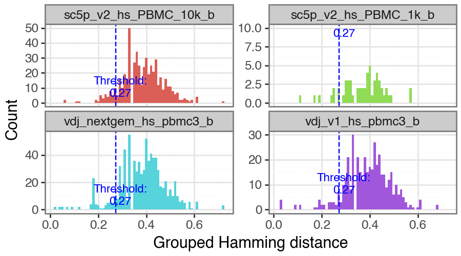
clone distance threshold: 0.2806603008124624
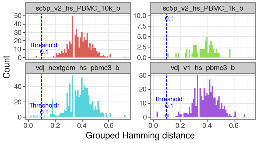
You can also manually select a value as the threshold if you wish. Note that rerunning this with manual_threshold is just for reproducing the plot but with the line at 0.1 in this tutorial.
[10]:
_ = ddl.pp.calculate_threshold(vdj, manual_threshold=0.1)
Calculating threshold
R[write to console]: Error in (function (db, sequenceColumn = "junction", vCallColumn = "v_call",  :
  254 cell(s) with multiple heavy chains found. One heavy chain per cell is expected.
Rerun this after filtering. For now, switching to heavy mode.
R[write to console]: Running in non-single-cell mode.
We can run ddl.tl.define_clones to call changeo’s DefineClones.py; see here for more info. The value in dist option (corresponds to threshold value) needs to be manually supplied. Additional options for ddl.tl.define_clones to provide to DefineClones.py can be supplied as a list to the additional_args option.
[11]:
# make a copy of the original vdj object to compare results
vdj_changeo = vdj.copy()
ddl.tl.define_clones(vdj_changeo, dist=threshold, key_added="changeo_clone_id")
vdj_changeo
Finding clones
Running command: DefineClones.py -d /var/folders/_r/j_8_fj3x28n2th3ch0ckn9c40000gt/T/tmpa5tqo7fx/tmp/dandelion_define_clones_heavy-clone.tsv -o /var/folders/_r/j_8_fj3x28n2th3ch0ckn9c40000gt/T/tmpa5tqo7fx/dandelion_define_clones_heavy-clone.tsv --act set --model ham --norm len --dist 0.2806603008124624 --nproc 1 --vf v_call_genotyped

       START> DefineClones
        FILE> dandelion_define_clones_heavy-clone.tsv
   SEQ_FIELD> junction
     V_FIELD> v_call_genotyped
     J_FIELD> j_call
 MAX_MISSING> 0
GROUP_FIELDS> None
      ACTION> set
        MODE> gene
    DISTANCE> 0.2806603008124624
     LINKAGE> single
       MODEL> ham
        NORM> len
         SYM> avg
       NPROC> 1

PROGRESS> [Grouping sequences] 13:43:56 (2406) 0.0 min

PROGRESS> [Assigning clones] 13:43:58 |####################| 100% (2,406) 0.0 min

 OUTPUT> dandelion_define_clones_heavy-clone.tsv
 CLONES> 2241
RECORDS> 2406
   PASS> 2406
   FAIL> 0
    END> DefineClones

 finished: Updated DandelionPolars object:
   'data', contig-indexed AIRR table
   'metadata', cell-indexed observations table
 (0:00:08)
[11]:
Lazy Dandelion object with n_obs = 2496 and n_contigs = 5792
    data: sequence_id, sequence, rev_comp, productive, v_call, d_call, j_call, sequence_alignment, germline_alignment, junction, junction_aa, v_cigar, d_cigar, j_cigar, stop_codon, vj_in_frame, locus, junction_length, np1_length, np2_length, v_sequence_start, v_sequence_end, v_germline_start, v_germline_end, d_sequence_start, d_sequence_end, d_germline_start, d_germline_end, j_sequence_start, j_sequence_end, j_germline_start, j_germline_end, v_score, v_identity, v_support, d_score, d_identity, d_support, j_score, j_identity, j_support, fwr1, fwr2, fwr3, fwr4, cdr1, cdr2, cdr3, cell_id, consensus_count, umi_count, v_call_10x, d_call_10x, j_call_10x, junction_10x, junction_10x_aa, j_call_blastn, j_identity_blastn, j_alignment_length_blastn, j_number_of_mismatches_blastn, j_number_of_gap_openings_blastn, j_sequence_start_blastn, j_sequence_end_blastn, j_germline_start_blastn, j_germline_end_blastn, j_support_blastn, j_score_blastn, j_sequence_alignment_blastn, j_germline_alignment_blastn, j_call_igblastn, j_source, j_support_igblastn, j_score_igblastn, d_call_blastn, d_identity_blastn, d_alignment_length_blastn, d_number_of_mismatches_blastn, d_number_of_gap_openings_blastn, d_sequence_start_blastn, d_sequence_end_blastn, d_germline_start_blastn, d_germline_end_blastn, d_support_blastn, d_score_blastn, d_sequence_alignment_blastn, d_germline_alignment_blastn, d_call_igblastn, d_source, d_support_igblastn, d_score_igblastn, v_call_genotyped, germline_alignment_d_mask, sample_id, c_call, c_sequence_alignment, c_germline_alignment, c_sequence_start, c_sequence_end, c_score, c_identity, c_call_10x, junction_aa_length, fwr1_aa, fwr2_aa, fwr3_aa, fwr4_aa, cdr1_aa, cdr2_aa, cdr3_aa, sequence_alignment_aa, v_sequence_alignment_aa, d_sequence_alignment_aa, j_sequence_alignment_aa, complete_vdj, j_call_multimappers, j_call_multiplicity, j_call_sequence_start_multimappers, j_call_sequence_end_multimappers, j_call_support_multimappers, mu_count, rearrangement_status, v_call_functionality, d_call_functionality, j_call_functionality, extra, ambiguous, clone_id, changeo_clone_id
    metadata: cell_id, changeo_clone_id, changeo_clone_id_rank, sample_id, productive_VDJ, productive_VJ, d_call_VDJ, j_call_VDJ, j_call_VJ, junction_VDJ, junction_VJ, junction_aa_VDJ, junction_aa_VJ, locus_VDJ, locus_VJ, v_call_VDJ, v_call_VJ, c_call_VDJ, c_call_VJ, umi_count_VDJ, umi_count_VJ, productive_VDJ_main, productive_VJ_main, d_call_VDJ_main, j_call_VDJ_main, j_call_VJ_main, junction_VDJ_main, junction_VJ_main, junction_aa_VDJ_main, junction_aa_VJ_main, locus_VDJ_main, locus_VJ_main, v_call_genotyped_VDJ_main, v_call_genotyped_VJ_main, c_call_VDJ_main, c_call_VJ_main, umi_count_VDJ_main, umi_count_VJ_main, isotype, isotype_main, isotype_status, locus_status, chain_status, rearrangement_status_VDJ, rearrangement_status_VJ
    distances: distance matrix of shape (2496, 2496)
Note that I specified the parameter key_added and this adds the clone id output from ddl.tl.define_clones into a separate column. If left as default (None), it will write into clone_id column. The same key_added parameter can be specified in ddl.tl.find_clones earlier. You will notice that vdj_changeo is initisalised with changeo_clone_id as the first column while vdj has clone_id.
Other clustering methods
dandelion also now supports clustering methods from scoper. You can access the functions through:
dandelion.external.immcancation.scoper.identical_clones(vdj, ...)
dandelion.external.immcancation.scoper.hierarchical_clones(vdj, ...)
dandelion.external.immcancation.scoper.spectral_clones(vdj, ...)
see the dandelion documentation for more information.
Generation of V(D)J network
dandelion generates a network to facilitate visualisation of results, inspired from [Bashford-Rogers2013]. The deafult uses the full V(D)J contig amino acid sequences to chart a tree-like network for each clone, but it can also be used on any sequence columns, e.g. junctional nucleotide sequences. The actual visualization of the network is in the next tutorial.
ddl.tl.generate_network now accepts and returns DandelionPolars objects.
Reusing pre-computed distances
generate_network now automatically detects the pre-computed distance matrix in vdj.distances at the start. If vdj.distances exists (generated by find_clones(store_distances=True)), the entire distance computation step is skipped. This is logged as “Using pre-computed distances from .distances”. If vdj.distances is None, the distances will be recomputed from scratch.
Layout Method Updates
Several new layout algorithm options are available:
Method |
Description |
|---|---|
|
Original Python modified Fruchterman-Reingold layout |
|
New default. Numba-accelerated FR layout (faster on CPU) |
|
PyTorch GPU-accelerated FR (auto-tiles for >100K nodes) |
|
Barnes-Hut O(N log N) CPU layout (scalable for large graphs) |
|
Barnes-Hut GPU layout (requires CUDA) |
|
ForceAtlas2 (requires |
The singleton_mass parameter (default 0.5) controls the mass of isolated nodes in Barnes-Hut layouts. Lowering this reduces the repulsive force that singletons exert on connected components.
Before proceeding, let’s do a bit of subsetting. Here I want to remove the Orphan VJ cells (lacking BCR heavy chain i.e. VDJ information). Whether or not you want to do this is up to you. I’m doing this because I want to focus on the BCR heavy chain for now. You may elect to keep everything and that can be your starting point for further analysis.
[12]:
vdj = vdj[
    vdj.metadata["chain_status"].is_in(
        ["Single pair", "Extra pair", "Extra pair-exception", "Orphan VDJ"]
    )
].copy()
vdj
[12]:
Lazy Dandelion object with n_obs = 2353 and n_contigs = 5625
    data: sequence_id, sequence, rev_comp, productive, v_call, d_call, j_call, sequence_alignment, germline_alignment, junction, junction_aa, v_cigar, d_cigar, j_cigar, stop_codon, vj_in_frame, locus, junction_length, np1_length, np2_length, v_sequence_start, v_sequence_end, v_germline_start, v_germline_end, d_sequence_start, d_sequence_end, d_germline_start, d_germline_end, j_sequence_start, j_sequence_end, j_germline_start, j_germline_end, v_score, v_identity, v_support, d_score, d_identity, d_support, j_score, j_identity, j_support, fwr1, fwr2, fwr3, fwr4, cdr1, cdr2, cdr3, cell_id, consensus_count, umi_count, v_call_10x, d_call_10x, j_call_10x, junction_10x, junction_10x_aa, j_call_blastn, j_identity_blastn, j_alignment_length_blastn, j_number_of_mismatches_blastn, j_number_of_gap_openings_blastn, j_sequence_start_blastn, j_sequence_end_blastn, j_germline_start_blastn, j_germline_end_blastn, j_support_blastn, j_score_blastn, j_sequence_alignment_blastn, j_germline_alignment_blastn, j_call_igblastn, j_source, j_support_igblastn, j_score_igblastn, d_call_blastn, d_identity_blastn, d_alignment_length_blastn, d_number_of_mismatches_blastn, d_number_of_gap_openings_blastn, d_sequence_start_blastn, d_sequence_end_blastn, d_germline_start_blastn, d_germline_end_blastn, d_support_blastn, d_score_blastn, d_sequence_alignment_blastn, d_germline_alignment_blastn, d_call_igblastn, d_source, d_support_igblastn, d_score_igblastn, v_call_genotyped, germline_alignment_d_mask, sample_id, c_call, c_sequence_alignment, c_germline_alignment, c_sequence_start, c_sequence_end, c_score, c_identity, c_call_10x, junction_aa_length, fwr1_aa, fwr2_aa, fwr3_aa, fwr4_aa, cdr1_aa, cdr2_aa, cdr3_aa, sequence_alignment_aa, v_sequence_alignment_aa, d_sequence_alignment_aa, j_sequence_alignment_aa, complete_vdj, j_call_multimappers, j_call_multiplicity, j_call_sequence_start_multimappers, j_call_sequence_end_multimappers, j_call_support_multimappers, mu_count, rearrangement_status, v_call_functionality, d_call_functionality, j_call_functionality, extra, ambiguous, clone_id
    metadata: cell_id, clone_id, clone_id_rank, sample_id, productive_VDJ, productive_VJ, d_call_VDJ, j_call_VDJ, j_call_VJ, junction_VDJ, junction_VJ, junction_aa_VDJ, junction_aa_VJ, locus_VDJ, locus_VJ, v_call_VDJ, v_call_VJ, c_call_VDJ, c_call_VJ, umi_count_VDJ, umi_count_VJ, productive_VDJ_main, productive_VJ_main, d_call_VDJ_main, j_call_VDJ_main, j_call_VJ_main, junction_VDJ_main, junction_VJ_main, junction_aa_VDJ_main, junction_aa_VJ_main, locus_VDJ_main, locus_VJ_main, v_call_genotyped_VDJ_main, v_call_genotyped_VJ_main, c_call_VDJ_main, c_call_VJ_main, umi_count_VDJ_main, umi_count_VJ_main, isotype, isotype_main, isotype_status, locus_status, chain_status, rearrangement_status_VDJ, rearrangement_status_VJ
    distances: distance matrix of shape (2353, 2353)
[ ]:
ddl.tl.generate_network(vdj, backend="networkx")
Generating network
Using pre-computed distances from .distances

Computing network layout
OMP: Info #276: omp_set_nested routine deprecated, please use omp_set_max_active_levels instead.
Computing expanded network layout
 finished.
   Updated Dandelion object
:    'layout', graph layout
 (0:00:00)
If you are dealing with a large dataset or very large clones, you may want to consider using igraph as the backend for network calculations. This is because networkx can be slow for large graphs. You can specify the backend by setting backend="igraph" in the function call.
At this point, we can save the dandelion object. We will visualise the network in the next tutorial.
[14]:
vdj.write_zipddl("dandelion_results_simplified.zipddl")
Full pairwise distance computation
With version 1.0.0, we are bringing back the option to compute the full pairwise distance matrix for every pair of cells. This is useful if you want to have a more comprehensive view of the relationships between cells, rather than just within clones. However, this can be quite memory intensive, especially for large datasets. For that purpose, we have refactored the distance computation to allow for parallelization, as well as with lazy evaluation using dask and zarr arrays, which allows
for handling larger datasets without running into memory issues. This is particularly useful when calculating the full pairwise distance matrix for every pair of cells, which can be quite memory-intensive. While this can also be used for distance_mode='clone', it’s incredibly slow. Its main advantage is for distance_mode='full' due to contigous nature of the distance matrix.
Note that with distance_mode='full', the required memory scales quadratically with the number of cells, so be cautious when using this option with large datasets. Using dask and zarr arrays can help mitigate this issue by allowing for out-of-core computation and parallel processing. This will create a zarr array on disk to store the distance matrix, which can later be read into memory in the DandelionPolars object with vdj.compute(), or specifying the path to the zarr
array when reading the DandelionPolars object with ddl.read_zipddl.
distance_mode Options
Mode |
Description |
|---|---|
|
Default. Computes distances only within clones. Memory efficient, suitable for most use cases. |
|
Computes full pairwise distances between all cells. Memory intensive — recommended to use with |
New Feature: Lazy Disk-Level Distance Computation
For large datasets, use lazy=True to offload distance computation to disk.
In lazy mode:
The distance matrix is stored as a Zarr array on disk, with a Dask lazy view on top.
vdj.distancesreturns adask.array.Arraythat computes on demand.Call
vdj.compute()to materialize it into an in-memory CSR sparse matrix.
zarr_path controls the storage location. If not specified, a temporary directory is created.
When pre-computed CSR distances are detected, lazy is automatically forced to False, since the CSR matrix is already in memory and disk-level lazy loading is unnecessary. You can run vdj.distances = None to delete the pre-computed CSR distances.
Finally, while pairwise distance computation is now possible, the final graph and layout is still based on within-clone distances only for performance reasons i.e. it will behave as before. In the future, we may explore options to incorporate full pairwise distances into the graph construction and visualization. We will demonstrate alternative ways to visualise the full pairwise distances in a later tutorial where use use UMAP and wnn on the full distance matrix.
To be able to use lazy=True, you need to have dask, zarr and distributed installed in your environment.
pip install "sc-dandelion[dask]"
Caveats with lazy distance matrix computation
With lazy=True, the distance matrix computation will be performed lazily on disk, which allows for handling larger datasets without running into memory issues. This is particularly useful when calculating the full pairwise distance matrix for every pair of cells, which can be quite memory-intensive.
While this can also be used for distance_mode='clone', it is not recommended for this mode as the distance matrix computation is already efficient enough for this mode.
This is also going to be slower than the in-memory computation for smaller datasets, so it’s generally recommended to use lazy=True only for larger datasets where memory constraints are a concern.
[15]:
# we will demonstrate one example here where we use the lazy method to compute the network
vdj_lazy = vdj.copy()
ddl.tl.generate_network(
    vdj_lazy,
    use_existing_distance=False,  # to overwrite the existing distance matrix
    use_existing_graph=False,
    distance_mode="full",
    lazy=True,
    n_cpus=8,
    zarr_path="distance_matrix.zarr",  # this is where the final computed distance matrix will be stored on disk
)
Generating network
Calculating distance matrix lazily with distance_mode = 'full'

Preparing distance matrix computation for 2353 sequences across 1 columns...
Auto-determined chunk size: 2353 (for 2353 sequences)
Dask client started: http://127.0.0.1:8787/status

Created Zarr array at: distance_matrix.zarr
Scattered DataFrame to workers
Starting computation of 1 chunks...
Merging temporary results into final Zarr array...
100%|██████████| 1/1 [00:00<00:00, 1.99it/s]
Computing network layout
Computing expanded network layout
 finished.
   Updated Dandelion object
:    'layout', graph layout
 (0:10:16)
[16]:
# view the vdj object
vdj_lazy
[16]:
Lazy Dandelion object with n_obs = 2353 and n_contigs = 5625
    data: sequence_id, sequence, rev_comp, productive, v_call, d_call, j_call, sequence_alignment, germline_alignment, junction, junction_aa, v_cigar, d_cigar, j_cigar, stop_codon, vj_in_frame, locus, junction_length, np1_length, np2_length, v_sequence_start, v_sequence_end, v_germline_start, v_germline_end, d_sequence_start, d_sequence_end, d_germline_start, d_germline_end, j_sequence_start, j_sequence_end, j_germline_start, j_germline_end, v_score, v_identity, v_support, d_score, d_identity, d_support, j_score, j_identity, j_support, fwr1, fwr2, fwr3, fwr4, cdr1, cdr2, cdr3, cell_id, consensus_count, umi_count, v_call_10x, d_call_10x, j_call_10x, junction_10x, junction_10x_aa, j_call_blastn, j_identity_blastn, j_alignment_length_blastn, j_number_of_mismatches_blastn, j_number_of_gap_openings_blastn, j_sequence_start_blastn, j_sequence_end_blastn, j_germline_start_blastn, j_germline_end_blastn, j_support_blastn, j_score_blastn, j_sequence_alignment_blastn, j_germline_alignment_blastn, j_call_igblastn, j_source, j_support_igblastn, j_score_igblastn, d_call_blastn, d_identity_blastn, d_alignment_length_blastn, d_number_of_mismatches_blastn, d_number_of_gap_openings_blastn, d_sequence_start_blastn, d_sequence_end_blastn, d_germline_start_blastn, d_germline_end_blastn, d_support_blastn, d_score_blastn, d_sequence_alignment_blastn, d_germline_alignment_blastn, d_call_igblastn, d_source, d_support_igblastn, d_score_igblastn, v_call_genotyped, germline_alignment_d_mask, sample_id, c_call, c_sequence_alignment, c_germline_alignment, c_sequence_start, c_sequence_end, c_score, c_identity, c_call_10x, junction_aa_length, fwr1_aa, fwr2_aa, fwr3_aa, fwr4_aa, cdr1_aa, cdr2_aa, cdr3_aa, sequence_alignment_aa, v_sequence_alignment_aa, d_sequence_alignment_aa, j_sequence_alignment_aa, complete_vdj, j_call_multimappers, j_call_multiplicity, j_call_sequence_start_multimappers, j_call_sequence_end_multimappers, j_call_support_multimappers, mu_count, rearrangement_status, v_call_functionality, d_call_functionality, j_call_functionality, extra, ambiguous, clone_id
    metadata: cell_id, clone_id, clone_id_rank, sample_id, productive_VDJ, productive_VJ, d_call_VDJ, j_call_VDJ, j_call_VJ, junction_VDJ, junction_VJ, junction_aa_VDJ, junction_aa_VJ, locus_VDJ, locus_VJ, v_call_VDJ, v_call_VJ, c_call_VDJ, c_call_VJ, umi_count_VDJ, umi_count_VJ, productive_VDJ_main, productive_VJ_main, d_call_VDJ_main, j_call_VDJ_main, j_call_VJ_main, junction_VDJ_main, junction_VJ_main, junction_aa_VDJ_main, junction_aa_VJ_main, locus_VDJ_main, locus_VJ_main, v_call_genotyped_VDJ_main, v_call_genotyped_VJ_main, c_call_VDJ_main, c_call_VJ_main, umi_count_VDJ_main, umi_count_VJ_main, isotype, isotype_main, isotype_status, locus_status, chain_status, rearrangement_status_VDJ, rearrangement_status_VJ
    layout: layout for 2353 vertices, layout for 148 vertices
    graph: networkx graph of 2353 vertices, networkx graph of 148 vertices
    distances: distance matrix of shape (2353, 2353)
[17]:
# save using the new default .zipddl format
vdj_lazy.write_zipddl("dandelion_results_lazy_distance_matrix.zipddl")
Because the distance matrix is lazy, it is not stored in the .zipddl file, but rather as the separate zarr array on disk in zarr_path. We will show you how to read this:
[18]:
# just specify the path to the distance_matirx.zarr that was created.
vdj_lazy_reload = ddl.read_zipddl(
    "dandelion_results_lazy_distance_matrix.zipddl",
    distance_zarr="distance_matrix.zarr",
)
vdj_lazy_reload
[18]:
Lazy Dandelion object with n_obs = 2353 and n_contigs = 5625
    data: sequence_id, sequence, rev_comp, productive, v_call, d_call, j_call, sequence_alignment, germline_alignment, junction, junction_aa, v_cigar, d_cigar, j_cigar, stop_codon, vj_in_frame, locus, junction_length, np1_length, np2_length, v_sequence_start, v_sequence_end, v_germline_start, v_germline_end, d_sequence_start, d_sequence_end, d_germline_start, d_germline_end, j_sequence_start, j_sequence_end, j_germline_start, j_germline_end, v_score, v_identity, v_support, d_score, d_identity, d_support, j_score, j_identity, j_support, fwr1, fwr2, fwr3, fwr4, cdr1, cdr2, cdr3, cell_id, consensus_count, umi_count, v_call_10x, d_call_10x, j_call_10x, junction_10x, junction_10x_aa, j_call_blastn, j_identity_blastn, j_alignment_length_blastn, j_number_of_mismatches_blastn, j_number_of_gap_openings_blastn, j_sequence_start_blastn, j_sequence_end_blastn, j_germline_start_blastn, j_germline_end_blastn, j_support_blastn, j_score_blastn, j_sequence_alignment_blastn, j_germline_alignment_blastn, j_call_igblastn, j_source, j_support_igblastn, j_score_igblastn, d_call_blastn, d_identity_blastn, d_alignment_length_blastn, d_number_of_mismatches_blastn, d_number_of_gap_openings_blastn, d_sequence_start_blastn, d_sequence_end_blastn, d_germline_start_blastn, d_germline_end_blastn, d_support_blastn, d_score_blastn, d_sequence_alignment_blastn, d_germline_alignment_blastn, d_call_igblastn, d_source, d_support_igblastn, d_score_igblastn, v_call_genotyped, germline_alignment_d_mask, sample_id, c_call, c_sequence_alignment, c_germline_alignment, c_sequence_start, c_sequence_end, c_score, c_identity, c_call_10x, junction_aa_length, fwr1_aa, fwr2_aa, fwr3_aa, fwr4_aa, cdr1_aa, cdr2_aa, cdr3_aa, sequence_alignment_aa, v_sequence_alignment_aa, d_sequence_alignment_aa, j_sequence_alignment_aa, complete_vdj, j_call_multimappers, j_call_multiplicity, j_call_sequence_start_multimappers, j_call_sequence_end_multimappers, j_call_support_multimappers, mu_count, rearrangement_status, v_call_functionality, d_call_functionality, j_call_functionality, extra, ambiguous, clone_id
    metadata: cell_id, clone_id, clone_id_rank, sample_id, productive_VDJ, productive_VJ, d_call_VDJ, j_call_VDJ, j_call_VJ, junction_VDJ, junction_VJ, junction_aa_VDJ, junction_aa_VJ, locus_VDJ, locus_VJ, v_call_VDJ, v_call_VJ, c_call_VDJ, c_call_VJ, umi_count_VDJ, umi_count_VJ, productive_VDJ_main, productive_VJ_main, d_call_VDJ_main, j_call_VDJ_main, j_call_VJ_main, junction_VDJ_main, junction_VJ_main, junction_aa_VDJ_main, junction_aa_VJ_main, locus_VDJ_main, locus_VJ_main, v_call_genotyped_VDJ_main, v_call_genotyped_VJ_main, c_call_VDJ_main, c_call_VJ_main, umi_count_VDJ_main, umi_count_VJ_main, isotype, isotype_main, isotype_status, locus_status, chain_status, rearrangement_status_VDJ, rearrangement_status_VJ
    layout: layout for 2353 vertices, layout for 148 vertices
    graph: networkx graph of 2353 vertices, networkx graph of 148 vertices
    distances: distance matrix of shape (2353, 2353)
[19]:
vdj_lazy_reload.distances
[19]:
|
||||||||||||||||
The distance matrix is read lazily as a dask.array.Array. To materialize the distance matrix into memory as a CSR sparse matrix, you can call vdj.compute(). Note that this will load the entire distance matrix into memory, so make sure you have enough RAM available.
[20]:
vdj_lazy_reload.compute()
vdj_lazy_reload.distances
[20]:
<Compressed Sparse Row sparse matrix of dtype 'float64'
        with 5536207 stored elements and shape (2353, 2353)>