Visualizing V(D)J data
Integration with scanpy
Now that we have both 1) a pre-processed V(D)J data in DandelionPolars object and 2) matching AnnData object, we can start finding clones and ‘integrate’ the results. All the V(D)J (AIRR) analyses files can be saved as .tsv format so that it can be used in other tools like immcantation, immunoarch, vdjtools, etc.
The results can also be ported into the AnnData object for access to more plotting functions provided through scanpy [Wolf2018].
[1]:
import os
import scanpy as sc
import pandas as pd
import dandelion as ddl

sc.settings.verbosity = 3

# change to tutorials directory
os.chdir("dandelion_tutorial")
Read in the previously saved files
I will work with the same example from the previous section since I have the AnnData object saved and vdj table filtered.
[2]:
adata = sc.read_h5ad("adata.h5ad")
adata
[2]:
AnnData object with n_obs × n_vars = 25063 × 1309
    obs: 'sample_id', 'n_genes', 'n_genes_by_counts', 'total_counts', 'total_counts_mt', 'pct_counts_mt', 'gmm_pct_count_clusters_keep', 'scrublet_score', 'is_doublet', 'filter_rna', 'has_contig', 'productive_VDJ', 'productive_VJ', 'd_call_VDJ', 'j_call_VDJ', 'j_call_VJ', 'junction_VDJ', 'junction_VJ', 'junction_aa_VDJ', 'junction_aa_VJ', 'locus_VDJ', 'locus_VJ', 'v_call_VDJ', 'v_call_VJ', 'c_call_VDJ', 'c_call_VJ', 'umi_count_VDJ', 'umi_count_VJ', 'productive_VDJ_main', 'productive_VJ_main', 'd_call_VDJ_main', 'j_call_VDJ_main', 'j_call_VJ_main', 'junction_VDJ_main', 'junction_VJ_main', 'junction_aa_VDJ_main', 'junction_aa_VJ_main', 'locus_VDJ_main', 'locus_VJ_main', 'v_call_genotyped_VDJ_main', 'v_call_genotyped_VJ_main', 'c_call_VDJ_main', 'c_call_VJ_main', 'umi_count_VDJ_main', 'umi_count_VJ_main', 'isotype', 'isotype_main', 'isotype_status', 'locus_status', 'chain_status', 'rearrangement_status_VDJ', 'rearrangement_status_VJ', 'leiden', 'clone_id', 'clone_id_rank'
    var: 'n_cells', 'highly_variable', 'means', 'dispersions', 'dispersions_norm', 'mean', 'std'
    uns: 'chain_status_colors', 'clone_id', 'dandelion', 'gex_neighbors', 'hvg', 'isotype_status_colors', 'leiden', 'leiden_colors', 'locus_status_colors', 'log1p', 'neighbors', 'pca', 'sample_id_colors', 'umap'
    obsm: 'X_pca', 'X_umap', 'X_vdj'
    varm: 'PCs'
    obsp: 'connectivities', 'distances'
[3]:
vdj = ddl.read_zipddl("dandelion_results_simplified.zipddl")
vdj
[3]:
Lazy Dandelion object with n_obs = 2353 and n_contigs = 5625
    data: sequence_id, sequence, rev_comp, productive, v_call, d_call, j_call, sequence_alignment, germline_alignment, junction, junction_aa, v_cigar, d_cigar, j_cigar, stop_codon, vj_in_frame, locus, junction_length, np1_length, np2_length, v_sequence_start, v_sequence_end, v_germline_start, v_germline_end, d_sequence_start, d_sequence_end, d_germline_start, d_germline_end, j_sequence_start, j_sequence_end, j_germline_start, j_germline_end, v_score, v_identity, v_support, d_score, d_identity, d_support, j_score, j_identity, j_support, fwr1, fwr2, fwr3, fwr4, cdr1, cdr2, cdr3, cell_id, consensus_count, umi_count, v_call_10x, d_call_10x, j_call_10x, junction_10x, junction_10x_aa, j_call_blastn, j_identity_blastn, j_alignment_length_blastn, j_number_of_mismatches_blastn, j_number_of_gap_openings_blastn, j_sequence_start_blastn, j_sequence_end_blastn, j_germline_start_blastn, j_germline_end_blastn, j_support_blastn, j_score_blastn, j_sequence_alignment_blastn, j_germline_alignment_blastn, j_call_igblastn, j_source, j_support_igblastn, j_score_igblastn, d_call_blastn, d_identity_blastn, d_alignment_length_blastn, d_number_of_mismatches_blastn, d_number_of_gap_openings_blastn, d_sequence_start_blastn, d_sequence_end_blastn, d_germline_start_blastn, d_germline_end_blastn, d_support_blastn, d_score_blastn, d_sequence_alignment_blastn, d_germline_alignment_blastn, d_call_igblastn, d_source, d_support_igblastn, d_score_igblastn, v_call_genotyped, germline_alignment_d_mask, sample_id, c_call, c_sequence_alignment, c_germline_alignment, c_sequence_start, c_sequence_end, c_score, c_identity, c_call_10x, junction_aa_length, fwr1_aa, fwr2_aa, fwr3_aa, fwr4_aa, cdr1_aa, cdr2_aa, cdr3_aa, sequence_alignment_aa, v_sequence_alignment_aa, d_sequence_alignment_aa, j_sequence_alignment_aa, complete_vdj, j_call_multimappers, j_call_multiplicity, j_call_sequence_start_multimappers, j_call_sequence_end_multimappers, j_call_support_multimappers, mu_count, rearrangement_status, v_call_functionality, d_call_functionality, j_call_functionality, extra, ambiguous, clone_id
    metadata: cell_id, clone_id, clone_id_rank, sample_id, productive_VDJ, productive_VJ, d_call_VDJ, j_call_VDJ, j_call_VJ, junction_VDJ, junction_VJ, junction_aa_VDJ, junction_aa_VJ, locus_VDJ, locus_VJ, v_call_VDJ, v_call_VJ, c_call_VDJ, c_call_VJ, umi_count_VDJ, umi_count_VJ, productive_VDJ_main, productive_VJ_main, d_call_VDJ_main, j_call_VDJ_main, j_call_VJ_main, junction_VDJ_main, junction_VJ_main, junction_aa_VDJ_main, junction_aa_VJ_main, locus_VDJ_main, locus_VJ_main, v_call_genotyped_VDJ_main, v_call_genotyped_VJ_main, c_call_VDJ_main, c_call_VJ_main, umi_count_VDJ_main, umi_count_VJ_main, isotype, isotype_main, isotype_status, locus_status, chain_status, rearrangement_status_VDJ, rearrangement_status_VJ
    layout: layout for 2353 vertices, layout for 148 vertices
    graph: networkx graph of 2353 vertices, networkx graph of 148 vertices
    distances: distance matrix of shape (2353, 2353)
ddl.tl.transfer
We can sync the V(D)J data from DandelionPolars object to the matching AnnData object using ddl.tl.transfer function.
[4]:
ddl.tl.transfer(adata, vdj)
adata
Transferring network
 finished: updated `.obs` with `.metadata`
wrote active layout to `.obsm['X_vdj']`; stashed all views in `.uns['dandelion']` ('X_vdj_all', 'X_vdj_expanded')
wrote `.obsp['connectivities']` & `['distances']` from graph[0]
stashed GEX matrices in `.uns['dandelion']` ('gex_connectivities', 'gex_distances')
stashed VDJ matrices in `.uns['dandelion']` under 'vdj_connectivities_all' / '_expanded'
added `.uns['clone_id']` clone-level mapping (0:00:00)
[4]:
AnnData object with n_obs × n_vars = 25063 × 1309
    obs: 'sample_id', 'n_genes', 'n_genes_by_counts', 'total_counts', 'total_counts_mt', 'pct_counts_mt', 'gmm_pct_count_clusters_keep', 'scrublet_score', 'is_doublet', 'filter_rna', 'has_contig', 'productive_VDJ', 'productive_VJ', 'd_call_VDJ', 'j_call_VDJ', 'j_call_VJ', 'junction_VDJ', 'junction_VJ', 'junction_aa_VDJ', 'junction_aa_VJ', 'locus_VDJ', 'locus_VJ', 'v_call_VDJ', 'v_call_VJ', 'c_call_VDJ', 'c_call_VJ', 'umi_count_VDJ', 'umi_count_VJ', 'productive_VDJ_main', 'productive_VJ_main', 'd_call_VDJ_main', 'j_call_VDJ_main', 'j_call_VJ_main', 'junction_VDJ_main', 'junction_VJ_main', 'junction_aa_VDJ_main', 'junction_aa_VJ_main', 'locus_VDJ_main', 'locus_VJ_main', 'v_call_genotyped_VDJ_main', 'v_call_genotyped_VJ_main', 'c_call_VDJ_main', 'c_call_VJ_main', 'umi_count_VDJ_main', 'umi_count_VJ_main', 'isotype', 'isotype_main', 'isotype_status', 'locus_status', 'chain_status', 'rearrangement_status_VDJ', 'rearrangement_status_VJ', 'leiden', 'clone_id', 'clone_id_rank'
    var: 'n_cells', 'highly_variable', 'means', 'dispersions', 'dispersions_norm', 'mean', 'std'
    uns: 'chain_status_colors', 'clone_id', 'dandelion', 'gex_neighbors', 'hvg', 'isotype_status_colors', 'leiden', 'leiden_colors', 'locus_status_colors', 'log1p', 'neighbors', 'pca', 'sample_id_colors', 'umap'
    obsm: 'X_pca', 'X_umap', 'X_vdj'
    varm: 'PCs'
    obsp: 'connectivities', 'distances'
Note
If a column with the same name between Dandelion.metadata and AnnData.obs already exists, tl.transfer will not overwrite the column in the AnnData object. This can be toggled to overwrite all with overwrite=True or overwrite=["column_name1", "column_name2"] if only some columns are to be overwritten.
You can see that AnnData object now contains a couple more columns in the .obs slot, corresponding to the metadata that is returned after tl.generate_network, and newly populated .obsm and .obsp slots. The original RNA connectivities and distances are now added into the .obsp slot as well.
Plotting in scanpy
pl.clone_network
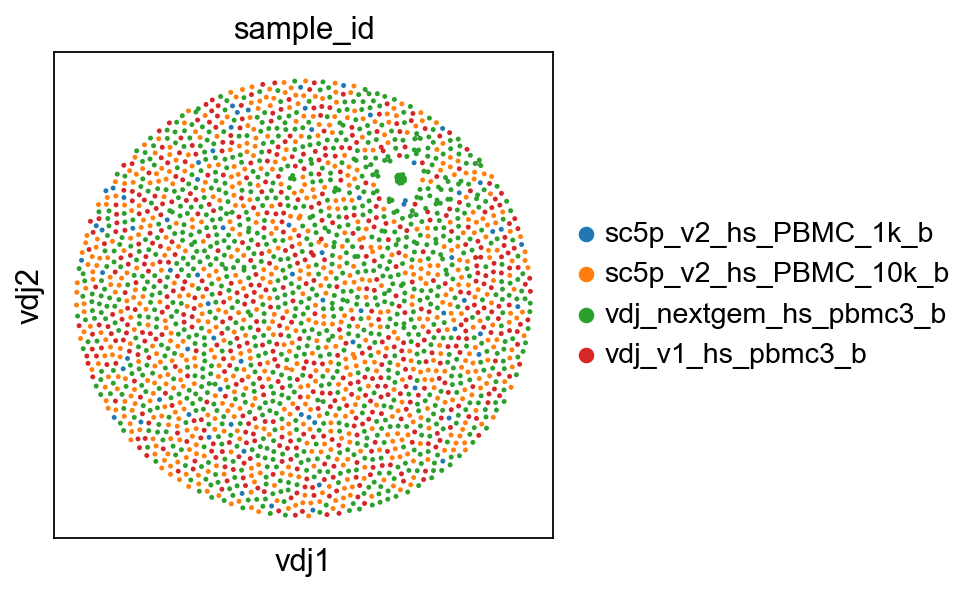
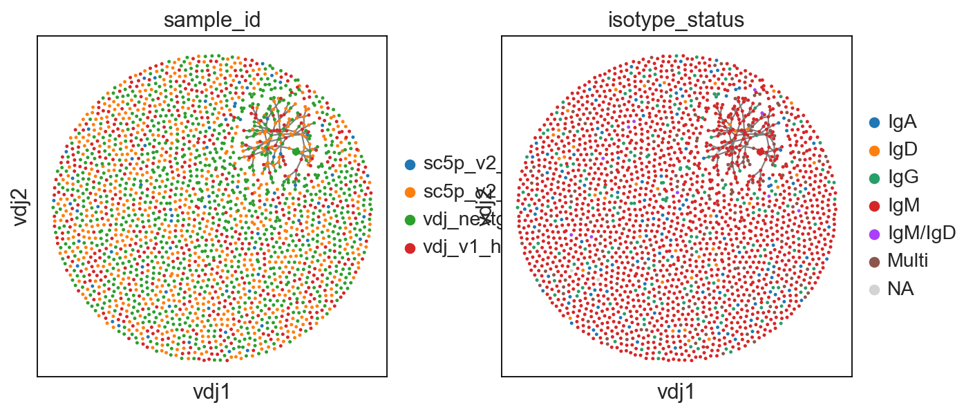
So now, basically we can plot in scanpy with their plotting modules. I’ve included a plotting function in dandelion, pl.clone_network, which is really just a wrapper of their pl.embedding module.
[5]:
sc.set_figure_params(figsize=[4, 4])
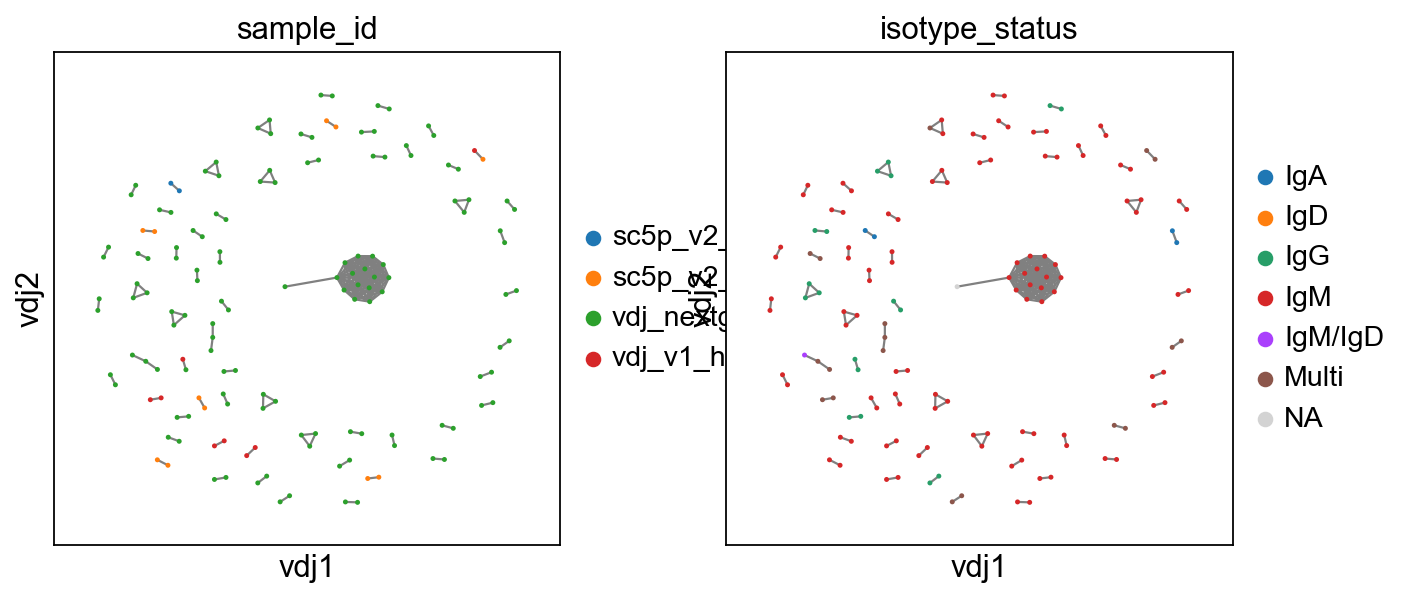
ddl.pl.clone_network(adata, color=["sample_id"], edges_width=1, size=20)

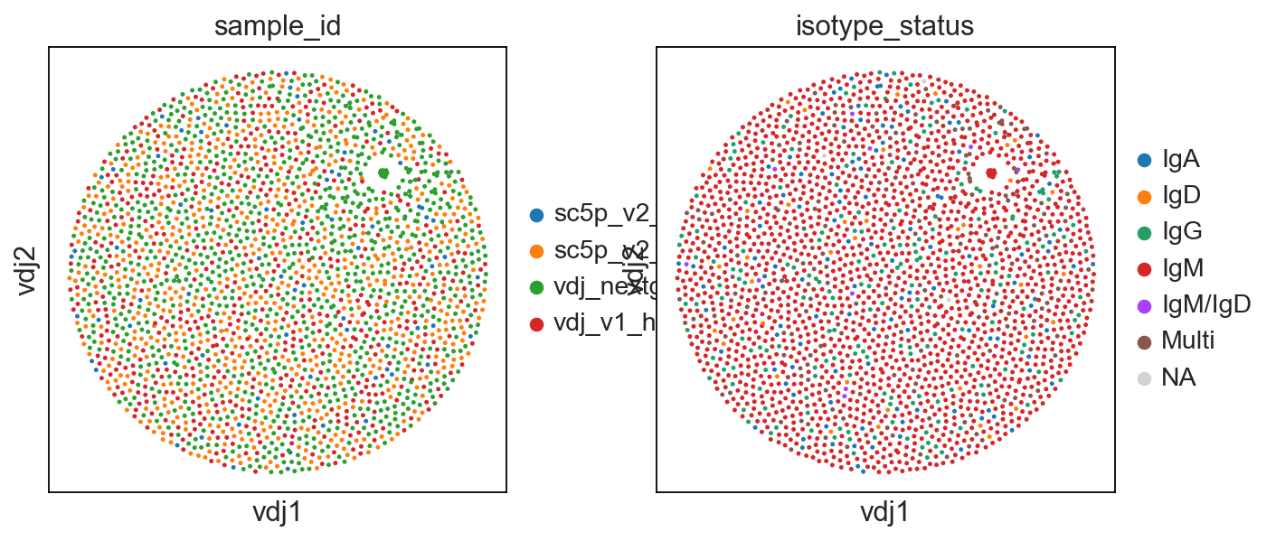
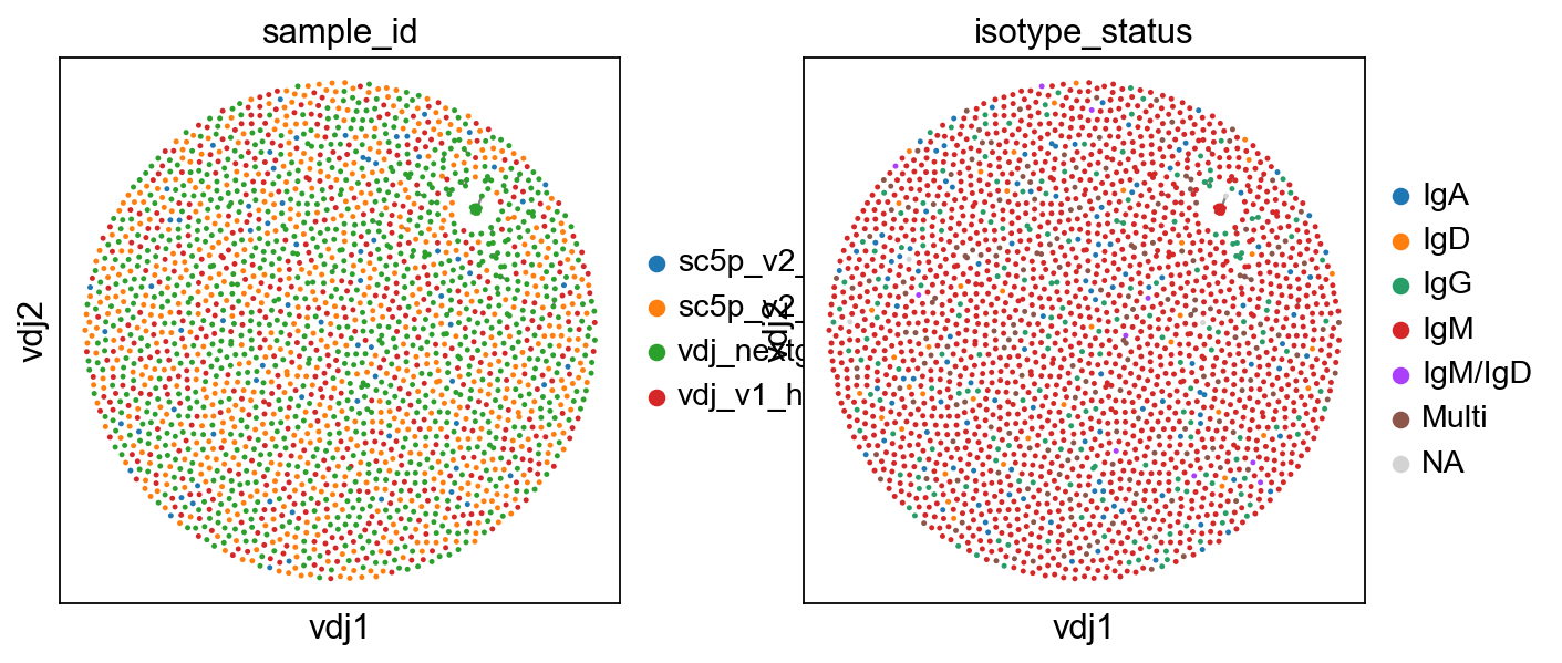
[6]:
ddl.pl.clone_network(
    adata, color=["sample_id", "isotype_status"], edges_width=1, size=20
)
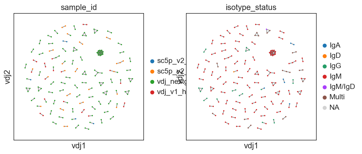
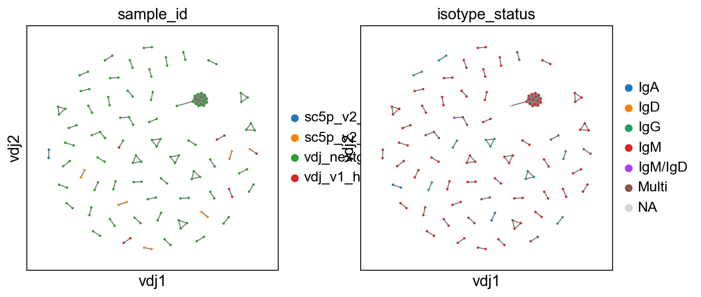
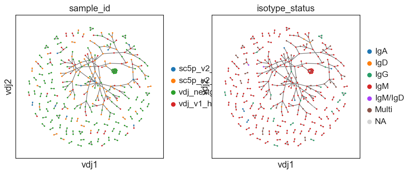
To show only expanded clones, we swap the view with a new function.
[7]:
ddl.tl.clone_view(adata, mode="expanded")
ddl.pl.clone_network(
    adata, color=["sample_id", "isotype_status"], edges_width=1, size=20
)
[8]:
# swap back to "all"
ddl.tl.clone_view(adata, mode="all")
ddl.pl.clone_network(adata, color=["sample_id"], edges_width=1, size=20)
The mode can also be swap to rna to reset the neighborhood graph to the RNA-based one for any downstream analysis. If mode is set to None, then the user can specify the keys in .obsp and .obsm to set as active by providing connectivities_key, distances_key, and embedding_key.
You might also be wondering why the plot for the largest clone looks different from the one we plotted in the base version of dandelion? In the base version, the clone had an additional edge to form a little sub-cluster, but in this plot, the clone is just a fully-connnected cluster.
This is because now the graph is based on the distances computed at the find_clones step, which uses the CDR3 junction as a default. With the full TCR/BCR sequence, it’s possible that there are more differences between the sequences, which results in a larger distance and thus no edge between some of the cells in the clone. Additionally, find_clones uses hamming distance as the default distance metric, which is different to the default distance metric used in generate_network
(levenshtein distance; which accounts for insertions and deletions). You can change the distance metric used in find_clones to levenshtein (or even BLOSUM62) to see if that results in different results.
For now, to reach a similar plot as the one we plotted in the base version, there are 2 options:
Run
find_clonesagain but usekey="sequence_alignment_aa"and potentially change the distance metric tolevenshteinorBLOSUM62to account for the full sequence differences, which will then be reflected in the graph structure in thegenerate_networkstep whenuse_existing_distance=True(which is the default).or, in the
generate_networkstep, useuse_existing_distance=Falseto re-compute the distance matrix based on the full sequence alignment (which is the defaultkey).
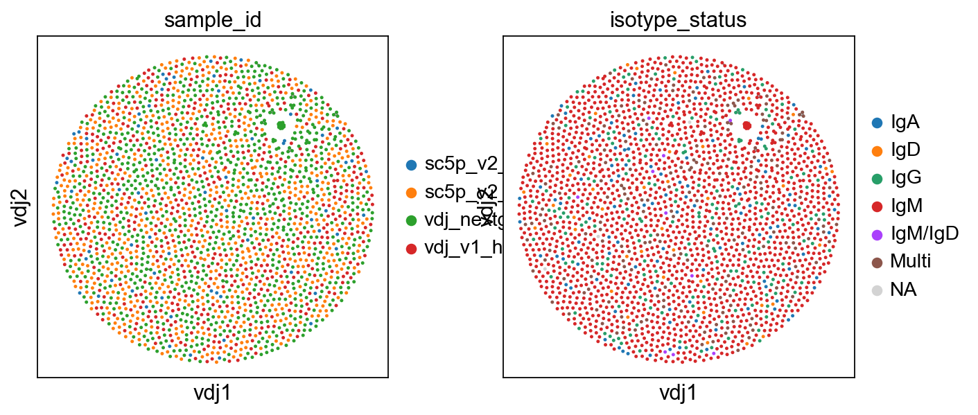
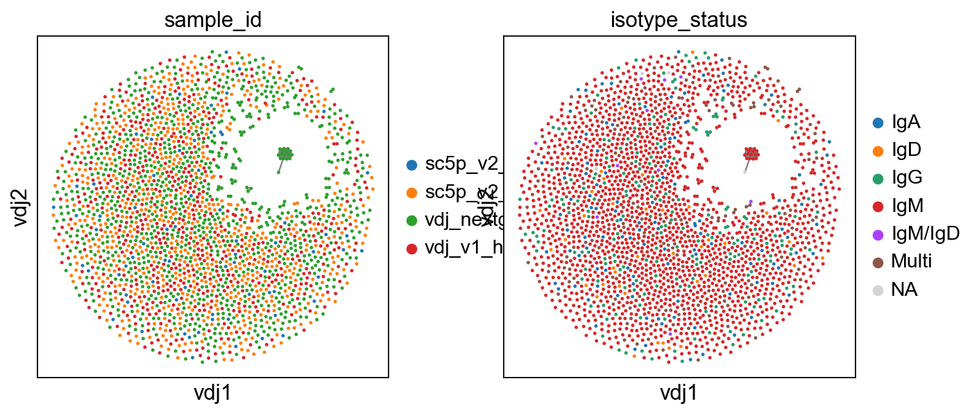
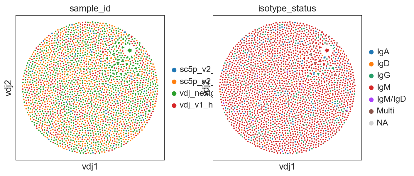
Let’s see how the second option works:
[9]:
# making a copy of both adata and vdj
vdj2 = vdj.copy()
adata2 = adata.copy()
# recompute layout with original method
ddl.tl.generate_network(
vdj2, use_existing_distance=False, use_existing_graph=False
)
ddl.tl.transfer(adata2, vdj2)
# visualise
ddl.pl.clone_network(
adata2, color=["sample_id", "isotype_status"], edges_width=1, size=20
)
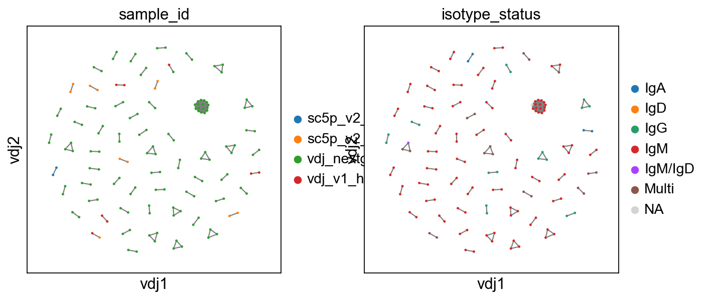
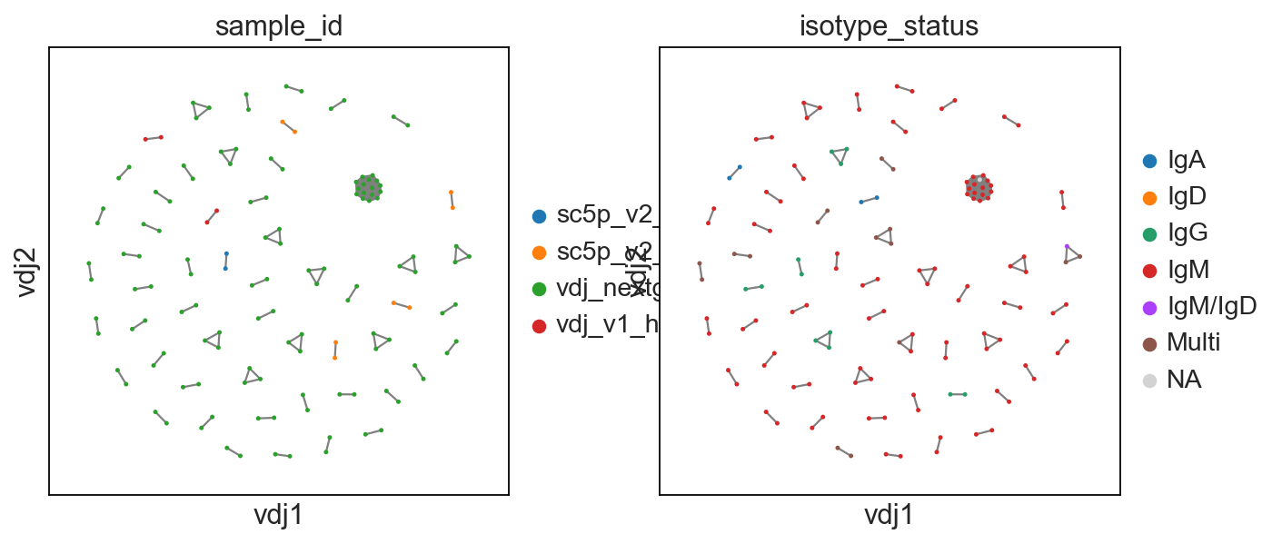
# swap to expanded mode.
ddl.tl.clone_view(adata2, mode="expanded")
# show where clones/clonotypes have more than 1 cell
ddl.pl.clone_network(
adata2, color=["sample_id", "isotype_status"], edges_width=1, size=20
)
Generating network
Calculating distance matrix  with distance_mode = 'clone'
100%|██████████| 2259/2259 [00:00<00:00, 906518.63it/s]
Distances calculated in 0.04 seconds
Computing network layout
OMP: Info #276: omp_set_nested routine deprecated, please use omp_set_max_active_levels instead.
Computing expanded network layout
 finished.
   Updated Dandelion object
:    'layout', graph layout
 (0:00:00)
Transferring network
 finished: updated `.obs` with `.metadata`
wrote active layout to `.obsm['X_vdj']`; stashed all views in `.uns['dandelion']` ('X_vdj_all', 'X_vdj_expanded')
wrote `.obsp['connectivities']` & `['distances']` from graph[0]
stashed GEX matrices in `.uns['dandelion']` ('gex_connectivities', 'gex_distances')
stashed VDJ matrices in `.uns['dandelion']` under 'vdj_connectivities_all' / '_expanded'
added `.uns['clone_id']` clone-level mapping (0:00:00)
Note
If you want a faster way to compute the layout for large graphs, you might want to try the mod_fr_bh layout method. Unlike the default mod_fr2 which uses a Numba-accelerated modified Fruchterman-Reingold algorithm, mod_fr_bh uses a Barnes-Hut approximation with O(N log N) complexity, making it more scalable for large datasets.
[10]:
# recompute layout with original method
ddl.tl.generate_network(vdj2, layout_method="mod_fr_bh")
ddl.tl.transfer(adata2, vdj2)
# visualise
ddl.pl.clone_network(
    adata2, color=["sample_id", "isotype_status"], edges_width=1, size=20
)
# swap to expanded mode.
ddl.tl.clone_view(adata2, mode="expanded")
# show where clones/clonotypes have more than 1 cell
ddl.pl.clone_network(
    adata2, color=["sample_id", "isotype_status"], edges_width=1, size=20
)
Generating network layout from pre-computed network
Computing network layout (Barnes-Hut CPU)
Computing expanded network layout (Barnes-Hut CPU)
 finished.
   Updated Dandelion object
:    'layout', graph layout
 (0:00:00)
Transferring network
 finished: updated `.obs` with `.metadata`
wrote active layout to `.obsm['X_vdj']`; stashed all views in `.uns['dandelion']` ('X_vdj_all', 'X_vdj_expanded')
wrote `.obsp['connectivities']` & `['distances']` from graph[0]
stashed GEX matrices in `.uns['dandelion']` ('gex_connectivities', 'gex_distances')
stashed VDJ matrices in `.uns['dandelion']` under 'vdj_connectivities_all' / '_expanded'
added `.uns['clone_id']` clone-level mapping (0:00:00)
tl.extract_edge_weights
We provide an edge weight extractor tool tl.extract_edge_weights to retrieve the edge weights that can be used to specify the edge widths according to weight/distance.
[11]:
# To illustrate this, first recompute the graph by specifying a minimum size
vdjx = vdj2.copy()
adatax = adata2.copy()
ddl.tl.generate_network(
    vdjx, min_size=3
)  # second graph will only contain clones/clonotypes with >= 3 cells
ddl.tl.transfer(adatax, vdjx)
edgeweights = [
    1 / (e + 1) for e in ddl.tl.extract_edge_weights(vdjx)
]  # invert and add 1 to each edge weight (e) so that distance of 0 becomes the thickest edge.
# therefore, the thicker the line, the shorter the edit distance.
ddl.tl.clone_view(adatax, mode="expanded")
ddl.pl.clone_network(
    adatax,
    color=["isotype_status"],
    legend_fontoutline=3,
    edges_width=edgeweights,
    size=50,
)
Generating network
Using pre-computed distances from .distances

Computing network layout
Computing expanded network layout
 finished.
   Updated Dandelion object
:    'layout', graph layout
 (0:00:00)
Transferring network
 finished: updated `.obs` with `.metadata`
wrote active layout to `.obsm['X_vdj']`; stashed all views in `.uns['dandelion']` ('X_vdj_all', 'X_vdj_expanded')
wrote `.obsp['connectivities']` & `['distances']` from graph[0]
stashed GEX matrices in `.uns['dandelion']` ('gex_connectivities', 'gex_distances')
stashed VDJ matrices in `.uns['dandelion']` under 'vdj_connectivities_all' / '_expanded'
added `.uns['clone_id']` clone-level mapping (0:00:00)
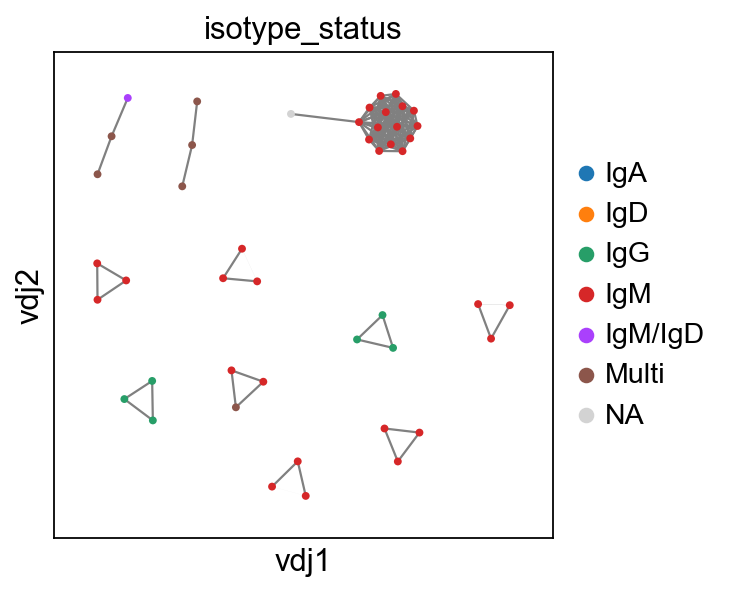
None here means there is no isotype information i.e. no c_call. If No_contig appears, it means there’s no V(D)J information.
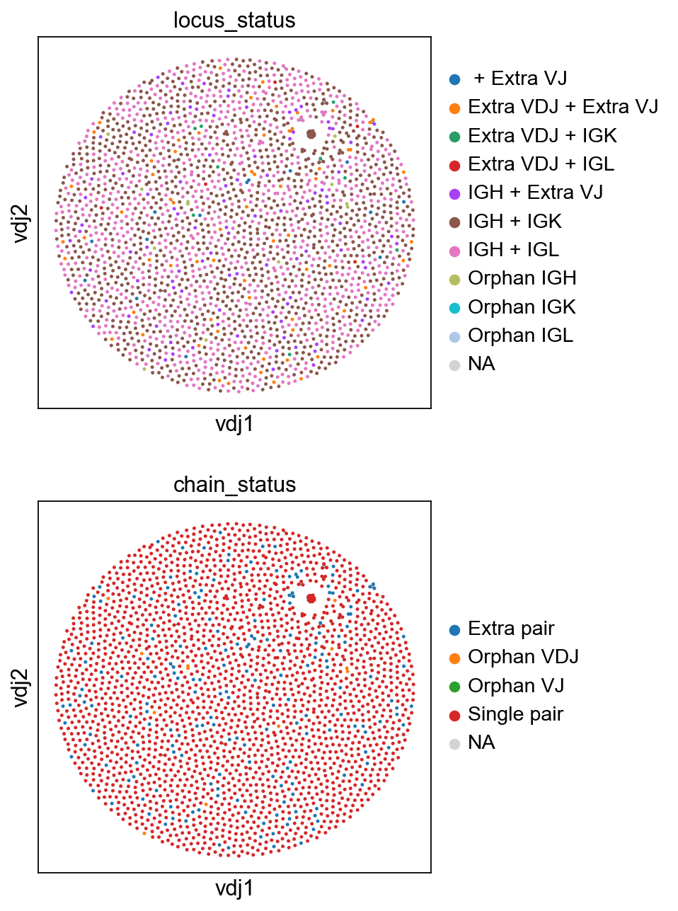
You can interact with pl.clone_network just as how you interact with the rest of the scatterplot modules in scanpy.
[12]:
sc.set_figure_params(figsize=[4, 4.5])
ddl.pl.clone_network(
    adata,
    color=["locus_status", "chain_status"],
    ncols=1,
    legend_fontoutline=3,
    edges_width=1,
    size=20,
)
you should be able to save the adata object and interact with it as per normal.
[13]:
adata.write_h5ad("adata.h5ad", compression="gzip")
Calculating size of clones
ddl.tl.clone_size
Sometimes it’s useful to evaluate the size of the clone. Here ddl.tl.clone_size does a simple calculation to enable that. From version 1.0.0 onwards, this function has been refactored and now also returning as proportion and can handle groups. There are new outputs e.g. clone size bins for rare, small, medium etc. similar to scRepertoire!
[14]:
ddl.tl.clone_size(vdj)
vdj.metadata[
    ["clone_id_size", "clone_id_size_prop", "clone_id_size_category"]
].collect()
[14]:
| clone_id_size | clone_id_size_prop | clone_id_size_category |
|---|---|---|
| f64 | f64 | str |
| 1.0 | 0.000425 | "Small" |
| 1.0 | 0.000425 | "Small" |
| 1.0 | 0.000425 | "Small" |
| 1.0 | 0.000425 | "Small" |
| 1.0 | 0.000425 | "Small" |
| … | … | … |
| 1.0 | 0.000425 | "Small" |
| 1.0 | 0.000425 | "Small" |
| 1.0 | 0.000425 | "Small" |
| 1.0 | 0.000425 | "Small" |
| 1.0 | 0.000425 | "Small" |
[15]:
vdj.metadata.collect()["clone_id_size_category"].value_counts()
[15]:
| clone_id_size_category | count |
|---|---|
| str | u32 |
| null | 8 |
| "Small" | 2299 |
| "Medium" | 46 |
You can also compute the clone size within groups by providing the group_by argument.
[16]:
ddl.tl.clone_size(vdj, group_by="isotype_status")
[17]:
import pandas as pd

pd.crosstab(
    vdj.metadata.collect()["isotype_status"],
    vdj.metadata.collect()["clone_id_size_category"],
).apply(lambda r: r / r.sum() * 100, axis=1)
[17]:
| col_0 | Large | Medium | Small |
|---|---|---|---|
| row_0 | |||
| IgA | 3.478261 | 96.521739 | 0.000000 |
| IgD | 100.000000 | 0.000000 | 0.000000 |
| IgG | 9.183673 | 90.816327 | 0.000000 |
| IgM | 0.000000 | 5.875831 | 94.124169 |
| IgM/IgD | 100.000000 | 0.000000 | 0.000000 |
| Multi | 9.604520 | 90.395480 | 0.000000 |
[18]:
ddl.tl.transfer(adata, vdj)
Transferring network
 finished: updated `.obs` with `.metadata`
wrote active layout to `.obsm['X_vdj']`; stashed all views in `.uns['dandelion']` ('X_vdj_all', 'X_vdj_expanded')
wrote `.obsp['connectivities']` & `['distances']` from graph[0]
stashed GEX matrices in `.uns['dandelion']` ('gex_connectivities', 'gex_distances')
stashed VDJ matrices in `.uns['dandelion']` under 'vdj_connectivities_all' / '_expanded'
added `.uns['clone_id']` clone-level mapping (0:00:00)
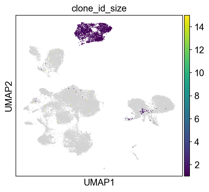
[19]:
sc.set_figure_params(figsize=[5, 4.5])
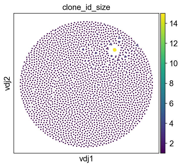
ddl.pl.clone_network(
adata,
color=["clone_id_size"],
legend_fontoutline=3,
edges_width=1,
size=20,
color_map="viridis",
)
sc.pl.umap(adata, color=["clone_id_size"], color_map="viridis")
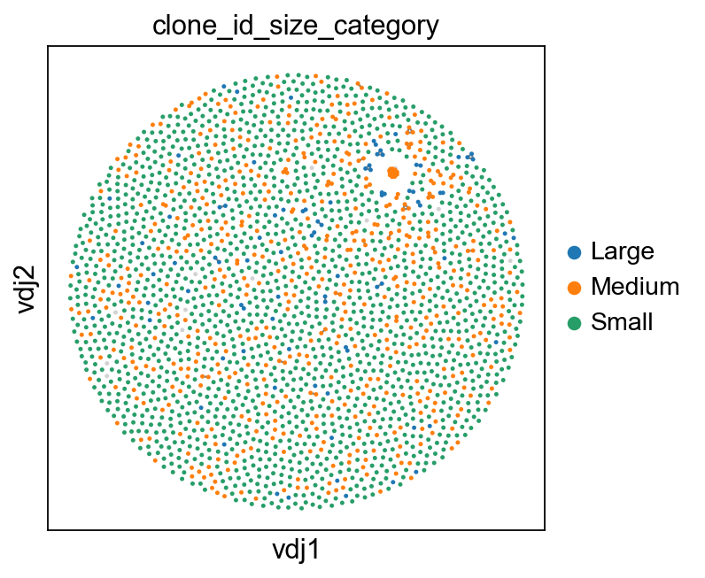
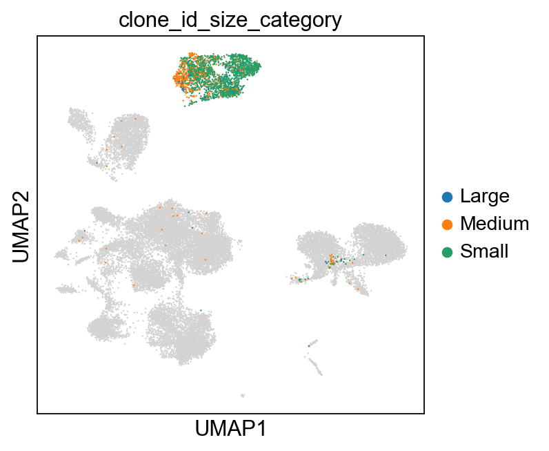
[20]:
sc.set_figure_params(figsize=[4.5, 4.5])
ddl.pl.clone_network(
    adata,
    color=["clone_id_size_category"],
    legend_fontoutline=3,
    edges_width=1,
    size=20,
    groups=["Small", "Medium", "Large", "Hyperexpanded"],
    na_in_legend=False,
)
sc.pl.umap(
    adata,
    color=["clone_id_size_category"],
    groups=["Small", "Medium", "Large", "Hyperexpanded"],
    na_in_legend=False,
)
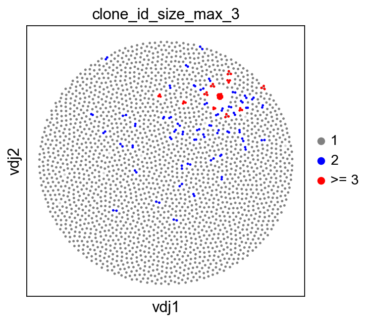
You can also specify max_size to clip off the calculation at a fixed value.
[21]:
ddl.tl.clone_size(vdj, max_size=3)
ddl.tl.transfer(adata, vdj)
Transferring network
 finished: updated `.obs` with `.metadata`
wrote active layout to `.obsm['X_vdj']`; stashed all views in `.uns['dandelion']` ('X_vdj_all', 'X_vdj_expanded')
wrote `.obsp['connectivities']` & `['distances']` from graph[0]
stashed GEX matrices in `.uns['dandelion']` ('gex_connectivities', 'gex_distances')
stashed VDJ matrices in `.uns['dandelion']` under 'vdj_connectivities_all' / '_expanded'
added `.uns['clone_id']` clone-level mapping (0:00:00)
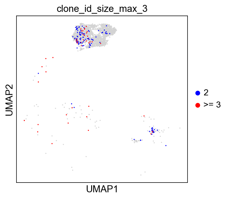
[22]:
sc.set_figure_params(figsize=[4.5, 4.5])
ddl.pl.clone_network(
    adata,
    color=["clone_id_size_max_3"],
    ncols=2,
    legend_fontoutline=3,
    edges_width=1,
    palette=["grey", "blue", "red"],
    size=20,
    na_in_legend=False,
)
sc.pl.umap(
    adata[adata.obs["has_contig"] == "True"],
    color=["clone_id_size_max_3"],
    groups=["2", ">= 3"],
    size=10,
    na_in_legend=False,
)
Additional plotting functions
ddl.pl.barplot
pl.barplot is a generic barplot function that will plot items in the metadata slot as a bar plot. This function will also interact with .obs slot if a scanpy object is used in place of DandelionPolars object. However, if your scanpy object holds a lot of non-B cells, then the plotting will be just be saturated with nan values.
Let’s first slice the DandelionPolars object to only include cells with at most one heavy chain.
[23]:
vdj_subset = vdj[
    vdj.metadata["chain_status"].is_in(["Single pair", "Orphan VDJ"])
]
vdj_subset
[23]:
Lazy Dandelion object with n_obs = 2158 and n_contigs = 4921
    data: sequence_id, sequence, rev_comp, productive, v_call, d_call, j_call, sequence_alignment, germline_alignment, junction, junction_aa, v_cigar, d_cigar, j_cigar, stop_codon, vj_in_frame, locus, junction_length, np1_length, np2_length, v_sequence_start, v_sequence_end, v_germline_start, v_germline_end, d_sequence_start, d_sequence_end, d_germline_start, d_germline_end, j_sequence_start, j_sequence_end, j_germline_start, j_germline_end, v_score, v_identity, v_support, d_score, d_identity, d_support, j_score, j_identity, j_support, fwr1, fwr2, fwr3, fwr4, cdr1, cdr2, cdr3, cell_id, consensus_count, umi_count, v_call_10x, d_call_10x, j_call_10x, junction_10x, junction_10x_aa, j_call_blastn, j_identity_blastn, j_alignment_length_blastn, j_number_of_mismatches_blastn, j_number_of_gap_openings_blastn, j_sequence_start_blastn, j_sequence_end_blastn, j_germline_start_blastn, j_germline_end_blastn, j_support_blastn, j_score_blastn, j_sequence_alignment_blastn, j_germline_alignment_blastn, j_call_igblastn, j_source, j_support_igblastn, j_score_igblastn, d_call_blastn, d_identity_blastn, d_alignment_length_blastn, d_number_of_mismatches_blastn, d_number_of_gap_openings_blastn, d_sequence_start_blastn, d_sequence_end_blastn, d_germline_start_blastn, d_germline_end_blastn, d_support_blastn, d_score_blastn, d_sequence_alignment_blastn, d_germline_alignment_blastn, d_call_igblastn, d_source, d_support_igblastn, d_score_igblastn, v_call_genotyped, germline_alignment_d_mask, sample_id, c_call, c_sequence_alignment, c_germline_alignment, c_sequence_start, c_sequence_end, c_score, c_identity, c_call_10x, junction_aa_length, fwr1_aa, fwr2_aa, fwr3_aa, fwr4_aa, cdr1_aa, cdr2_aa, cdr3_aa, sequence_alignment_aa, v_sequence_alignment_aa, d_sequence_alignment_aa, j_sequence_alignment_aa, complete_vdj, j_call_multimappers, j_call_multiplicity, j_call_sequence_start_multimappers, j_call_sequence_end_multimappers, j_call_support_multimappers, mu_count, rearrangement_status, v_call_functionality, d_call_functionality, j_call_functionality, extra, ambiguous, clone_id
    metadata: cell_id, clone_id, clone_id_rank, sample_id, productive_VDJ, productive_VJ, d_call_VDJ, j_call_VDJ, j_call_VJ, junction_VDJ, junction_VJ, junction_aa_VDJ, junction_aa_VJ, locus_VDJ, locus_VJ, v_call_VDJ, v_call_VJ, c_call_VDJ, c_call_VJ, umi_count_VDJ, umi_count_VJ, productive_VDJ_main, productive_VJ_main, d_call_VDJ_main, j_call_VDJ_main, j_call_VJ_main, junction_VDJ_main, junction_VJ_main, junction_aa_VDJ_main, junction_aa_VJ_main, locus_VDJ_main, locus_VJ_main, v_call_genotyped_VDJ_main, v_call_genotyped_VJ_main, c_call_VDJ_main, c_call_VJ_main, umi_count_VDJ_main, umi_count_VJ_main, isotype, isotype_main, isotype_status, locus_status, chain_status, rearrangement_status_VDJ, rearrangement_status_VJ, clone_id_size, clone_id_size_prop, clone_id_size_category, clone_id_size_max_3
    layout: layout for 2158 vertices, layout for 129 vertices
    graph: networkx graph of 2158 vertices, networkx graph of 129 vertices
    distances: distance matrix of shape (2158, 2158)
[24]:
import matplotlib as mpl
import matplotlib.pyplot as plt

mpl.rcParams.update(mpl.rcParamsDefault)

ddl.pl.barplot(
    vdj_subset,
    color="v_call_VDJ",
)
plt.show()
/Users/uqztuong/Documents/GitHub/dandelion/src/dandelion/polars/plotting/_plotting.py:153: FutureWarning:

Passing `palette` without assigning `hue` is deprecated and will be removed in v0.14.0. Assign the `x` variable to `hue` and set `legend=False` for the same effect.
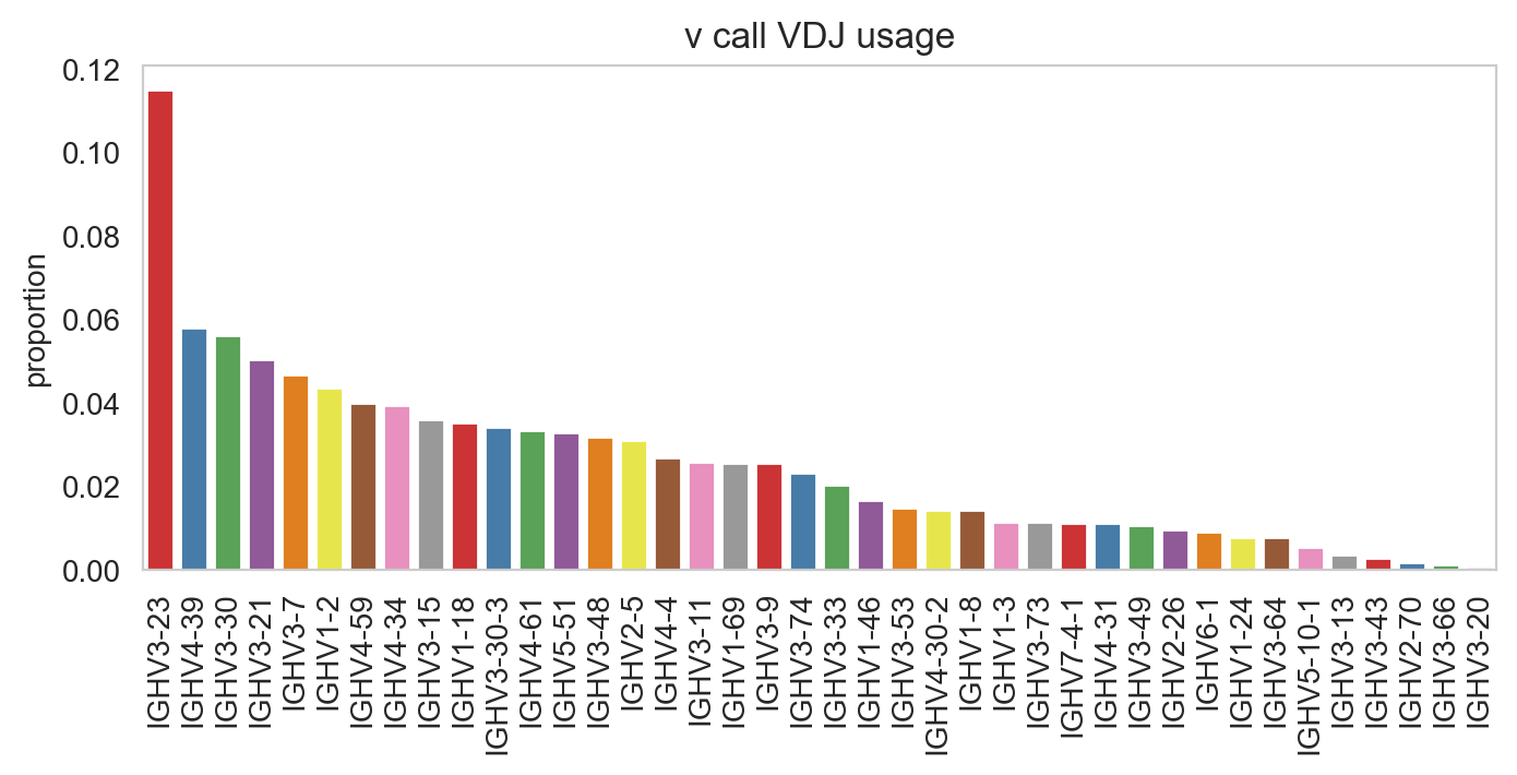
You can prevent it from sorting by specifying sort_descending = None. Colours can be changed with palette option.
[25]:
ddl.pl.barplot(
    vdj_subset,
    color="v_call_VDJ",
    sort_descending=None,
    palette="tab20",
)
plt.show()
/Users/uqztuong/Documents/GitHub/dandelion/src/dandelion/polars/plotting/_plotting.py:153: FutureWarning:

Passing `palette` without assigning `hue` is deprecated and will be removed in v0.14.0. Assign the `x` variable to `hue` and set `legend=False` for the same effect.
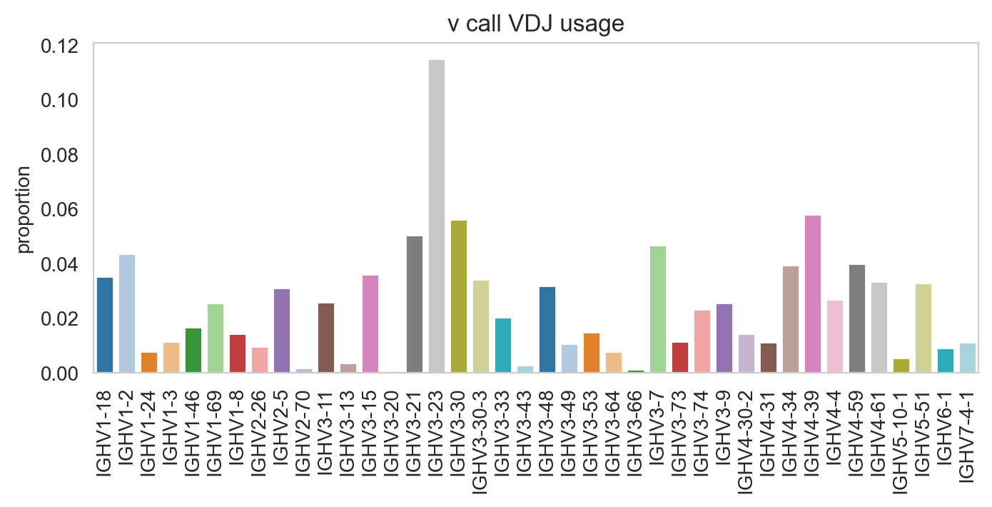
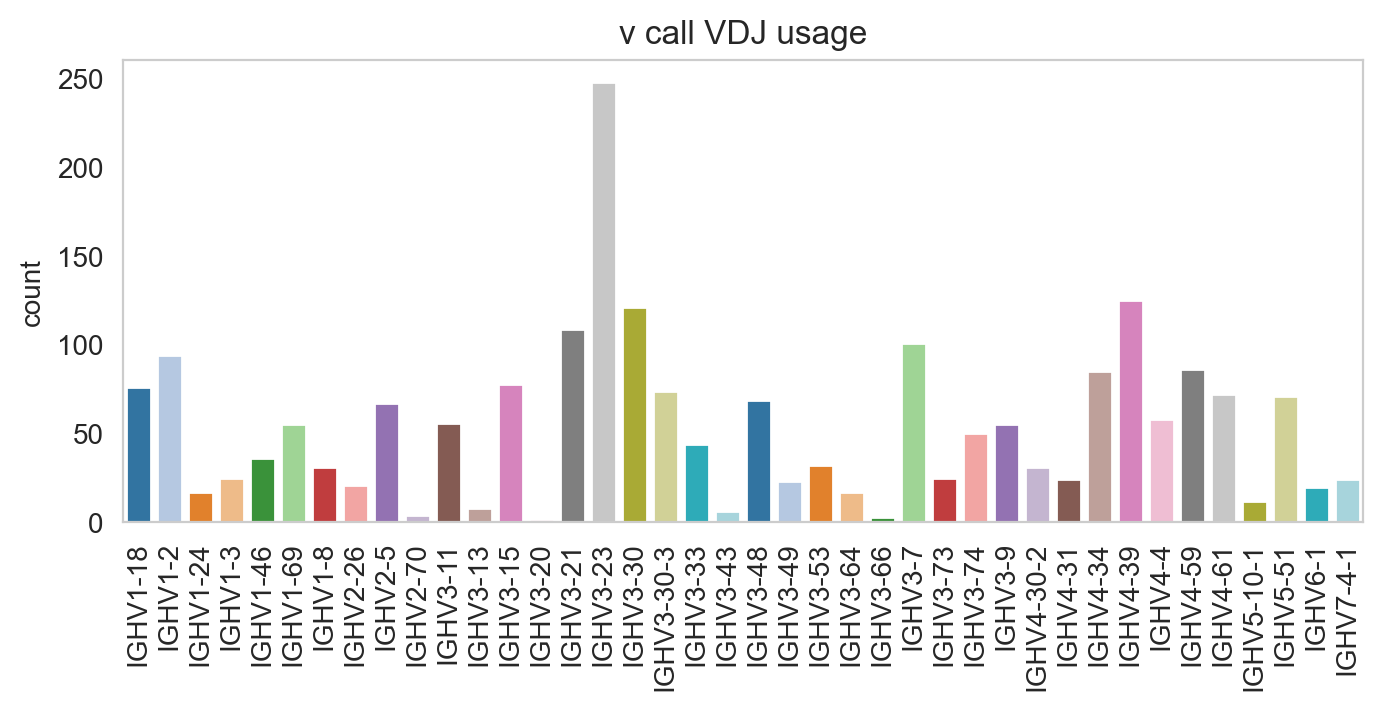
Specifying normalize = False will change the y-axis to counts.
[26]:
ddl.pl.barplot(
    vdj_subset,
    color="v_call_VDJ",
    normalize=False,
    sort_descending=None,
    palette="tab20",
)
plt.show()
/Users/uqztuong/Documents/GitHub/dandelion/src/dandelion/polars/plotting/_plotting.py:153: FutureWarning:

Passing `palette` without assigning `hue` is deprecated and will be removed in v0.14.0. Assign the `x` variable to `hue` and set `legend=False` for the same effect.
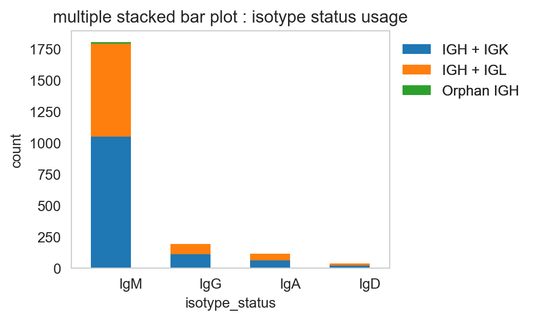
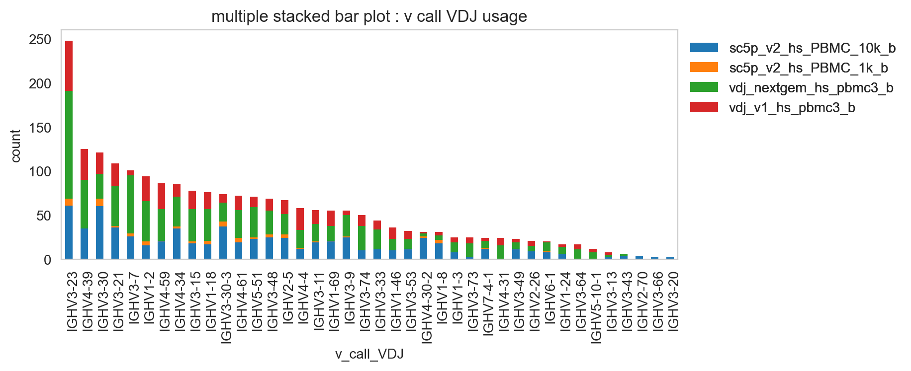
pl.stackedbarplot
pl.stackedbarplot is similar to above but can split between specified groups. Some examples below:
[27]:
ddl.pl.stackedbarplot(
    vdj_subset,
    color="isotype_status",
    group_by="locus_status",
    xtick_rotation=0,
    figsize=(4, 3),
)
plt.legend(bbox_to_anchor=(1, 1), loc="upper left", frameon=False)
plt.show()
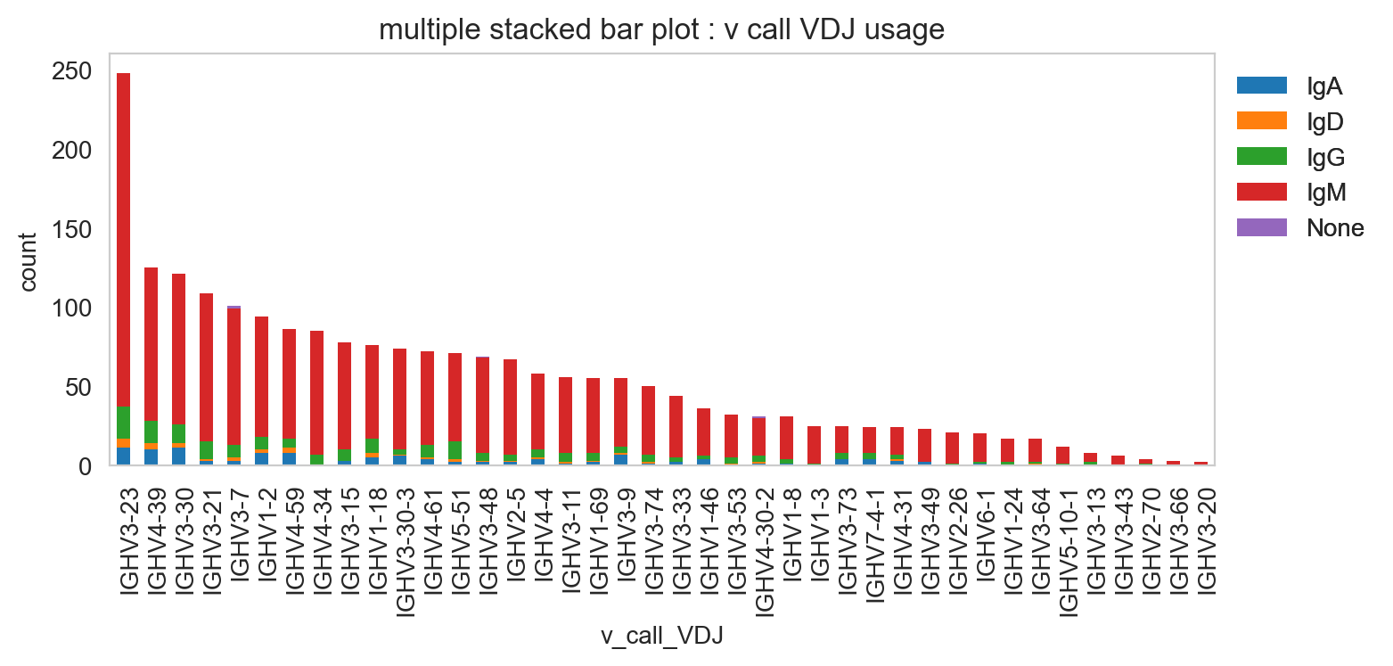
[28]:
ddl.pl.stackedbarplot(
    vdj_subset,
    color="v_call_VDJ",
    group_by="isotype_status",
)
plt.legend(bbox_to_anchor=(1, 1), loc="upper left", frameon=False)
plt.show()
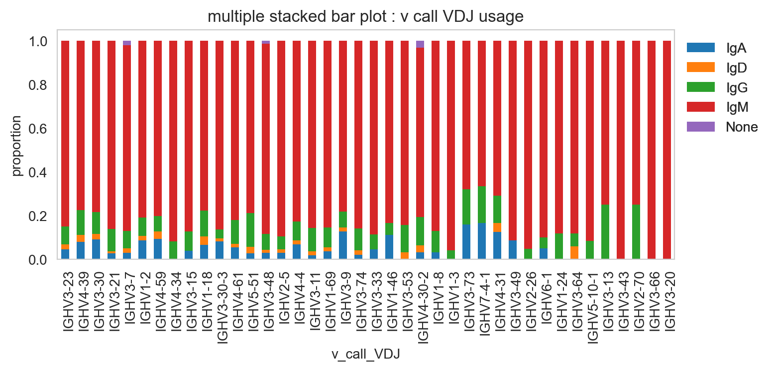
[29]:
ddl.pl.stackedbarplot(
    vdj_subset,
    color="v_call_VDJ",
    group_by="isotype_status",
    normalize=True,
)
plt.legend(bbox_to_anchor=(1, 1), loc="upper left", frameon=False)
plt.show()
[30]:
ddl.pl.stackedbarplot(
    vdj_subset,
    color="v_call_VDJ",
    group_by="chain_status",
)
plt.legend(bbox_to_anchor=(1, 1), loc="upper left", frameon=False)
plt.show()
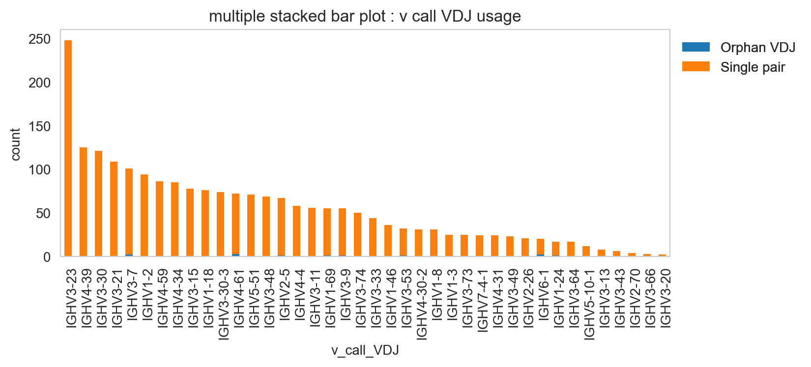
It’s obviously more useful if you don’t have too many groups, but you could try and plot everything and jiggle the legend options and color.
[31]:
ddl.pl.stackedbarplot(
    vdj_subset,
    color="v_call_VDJ",
    group_by="sample_id",
)
plt.legend(bbox_to_anchor=(1, 1), loc="upper left", frameon=False)
plt.show()
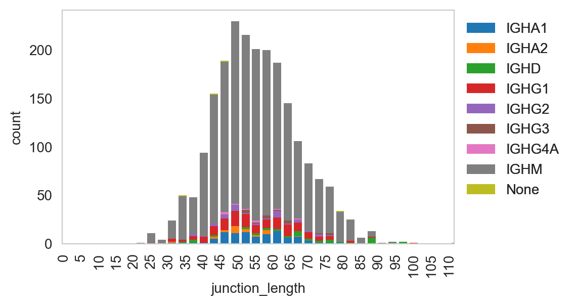
ddl.pl.spectratype
Spectratype plots contain info displaying CDR3 length distribution for specified groups. For this function, the current method only works for Dandelion and DandelionPolars objects as it requires access to the contig-indexed .data slot.
[32]:
ddl.pl.spectratype(
    vdj_subset,
    color="junction_length",
    group_by="c_call",
    locus="IGH",
    width=2.3,
)
plt.legend(bbox_to_anchor=(1, 1), loc="upper left", frameon=False)
plt.show()
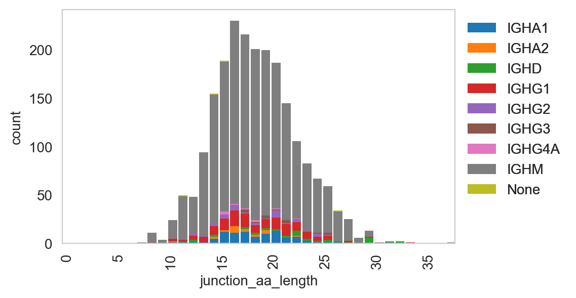
[33]:
ddl.pl.spectratype(
    vdj_subset,
    color="junction_aa_length",
    group_by="c_call",
    locus="IGH",
)
plt.legend(bbox_to_anchor=(1, 1), loc="upper left", frameon=False)
plt.show()
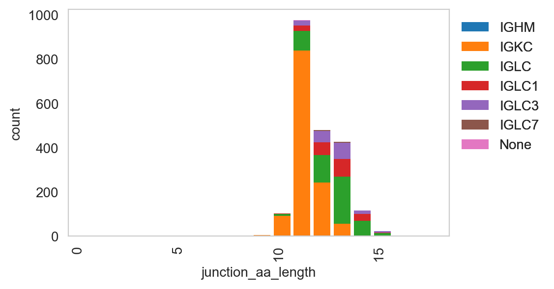
[34]:
ddl.pl.spectratype(
    vdj_subset,
    color="junction_aa_length",
    group_by="c_call",
    locus=["IGK", "IGL"],
)
plt.legend(bbox_to_anchor=(1, 1), loc="upper left", frameon=False)
plt.show()
ddl.pl.clone_overlap
There is now a circos-style clone overlap function where it looks for whether different samples share a clone. If they do, an arc/connection will be drawn between them.
[35]:
ddl.tl.clone_overlap(adata, group_by="leiden")
Calculating clone overlap
 finished: Updated AnnData:
   'uns', clone overlap table (0:00:00)
[36]:
sc.set_figure_params(figsize=[6, 6])
ddl.pl.clone_overlap(adata, group_by="leiden")
plt.show()
/opt/homebrew/Caskroom/miniforge/base/envs/dandelion/lib/python3.12/site-packages/nxviz/annotate.py:68: FutureWarning: DataFrameGroupBy.apply operated on the grouping columns. This behavior is deprecated, and in a future version of pandas the grouping columns will be excluded from the operation. Either pass `include_groups=False` to exclude the groupings or explicitly select the grouping columns after groupby to silence this warning.
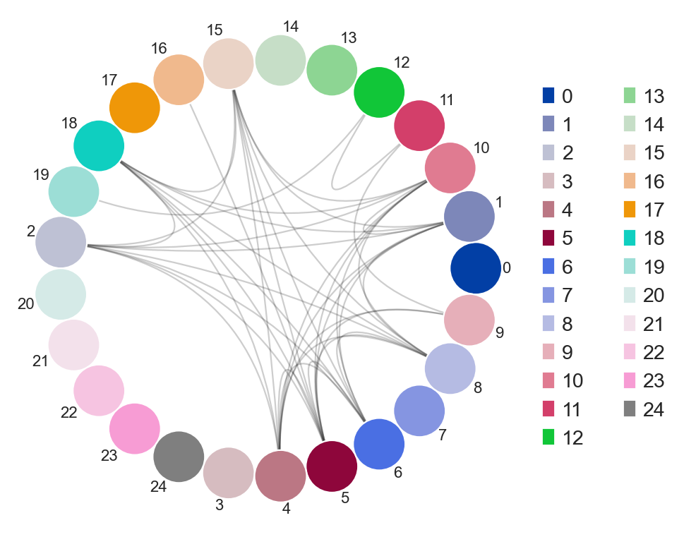
Other use cases for this would be, for example, to plot nodes as individual samples and the colors as group classifications of the samples. As long as this information is found in the .obs column in the AnnData, or even DandelionPolars.metadata, this will work.
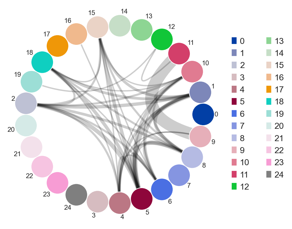
You an also specify weighted_overlap = True and the thickness of the edges will reflect the number of cells found to overlap between the nodes/samples.
[37]:
ddl.tl.clone_overlap(adata, group_by="leiden", weighted_overlap=True)
ddl.pl.clone_overlap(adata, group_by="leiden", weighted_overlap=True)
plt.show()
Calculating clone overlap
 finished: Updated AnnData:
   'uns', clone overlap table (0:00:00)
/opt/homebrew/Caskroom/miniforge/base/envs/dandelion/lib/python3.12/site-packages/nxviz/annotate.py:68: FutureWarning: DataFrameGroupBy.apply operated on the grouping columns. This behavior is deprecated, and in a future version of pandas the grouping columns will be excluded from the operation. Either pass `include_groups=False` to exclude the groupings or explicitly select the grouping columns after groupby to silence this warning.
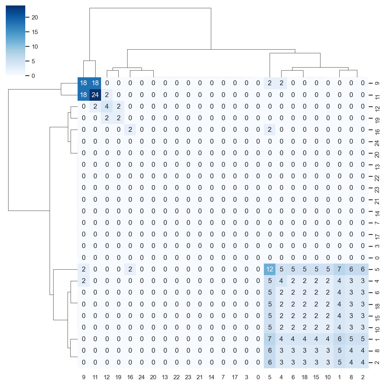
You can also visualise this as a heatmap by specifying as_heatmap = True.
[38]:
import seaborn as sns

sns.set(font_scale=0.8)

ddl.pl.clone_overlap(
    adata,
    group_by="leiden",
    weighted_overlap=True,
    as_heatmap=True,
    # seaborn clustermap kwargs
    cmap="Blues",
    annot=True,
    figsize=(8, 8),
    annot_kws={"size": 10},
    fmt="g",
)
plt.show()
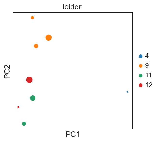
tl.vj_usage_pca
You can also compute the V/J gene usage in your various groups of interest. This function will return a new AnnData where instead of cells (obs) by gene (var), it will be group_by (obs) by V/J genes (var).
Note
This function now requires a DandelionPolars object as the vdj argument.
For example, I’m interested if the leiden clusters within each donor’s sample use V/J genes differently:
[39]:
# first make a concatenated group
adata.obs["sample_id_leiden"] = [
    s + "_" + l for s, l in zip(adata.obs["sample_id"], adata.obs["leiden"])
]
new_adata = ddl.tl.vj_usage_pca(
    adata,
    vdj,
    group_by="sample_id_leiden",
    mode="B",  # because B cells, use abT and gdT for alpha-beta and gamma-delta T cells respectively
    transfer_mapping=[
        "sample_id",
        "leiden",
    ],  # this transfers the sample_id and leiden values separately. if not provided, only sample_id_leiden is transferred.
    n_comps=3,  # 3 because the example is small here. the default is set at 30
)
new_adata
Computing PCA for V/J gene usage
computing PCA
    with n_comps=3
    finished (0:00:00)
 finished: Returned AnnData:
   'obsm', X_pca for V/J gene usage (0:00:00)
/opt/homebrew/Caskroom/miniforge/base/envs/dandelion/lib/python3.12/site-packages/scanpy/preprocessing/_pca/__init__.py:226: FutureWarning: Argument `use_highly_variable` is deprecated, consider using the mask argument. Use_highly_variable=True can be called through mask_var="highly_variable". Use_highly_variable=False can be called through mask_var=None
[39]:
AnnData object with n_obs × n_vars = 8 × 120
    obs: 'cell_type', 'cell_count', 'sample_id', 'leiden'
    uns: 'pca'
    obsm: 'X_pca'
    varm: 'PCs'
[40]:
sc.set_figure_params()

sc.pl.pca(new_adata, color="leiden", size=new_adata.obs["cell_count"])
# each dot is a `sample_id_leiden`. Check the .obs
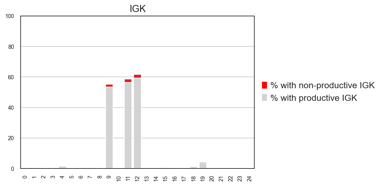
tl.productive_ratio/pl.productive_ratio
This new function lets you quantify what is the distribution of productive versus non-productive contigs at a cell-level. To do this, we need to re-check the DandelionPolars object so that non-productive columns are not removed.
[41]:
vdj2, adata2 = ddl.pp.check_contigs(vdj, adata, productive_only=False)
Filtering contigs...
Marking ambiguous contigs...
Initializing DandelionPolars object...
Transferring network
 finished: updated `.obs` with `.metadata`
 (0:00:00)
[42]:
ddl.tl.productive_ratio(adata2, vdj2, group_by="leiden", locus="IGK")
Tabulating productive ratio
 finished: Updated AnnData:
   'obs', 'IGK_productive'
   'uns', 'productive_ratio'
 (0:00:00)
[43]:
ddl.pl.productive_ratio(adata2, palette=["red", "lightgrey"])
plt.tight_layout()
# plt.savefig('plot.pdf')
plt.show()
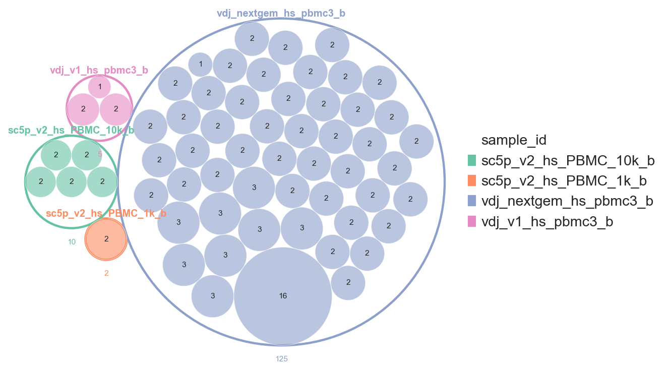
pl.clone_circlepackplot
pl.clone_circlepackplot is a bubble plot to visualise clone sizes within groups using circle packing. Each group (e.g. sample, celltype) is represented as an enclosing circle, with clones within that group shown as packed inner circles sized proportionally to clone size.
This function works with both AnnData and DandelionPolars objects. Singletons can be excluded by setting min_clone_size=2. We also enable show_count_labels=True to annotate each circle with its cell count.
[44]:
vdj.metadata.collect()["clone_id_size"].value_counts().sort("clone_id_size")
[44]:
| clone_id_size | count |
|---|---|
| f64 | u32 |
| null | 8 |
| 1.0 | 2197 |
| 2.0 | 102 |
| 3.0 | 30 |
| 16.0 | 16 |
[45]:
ddl.pl.clone_circlepackplot(
    vdj,
    group_by="sample_id",
    min_clone_size=2,
    show_count_labels=True,
    figsize=(7, 7),
)
plt.show()
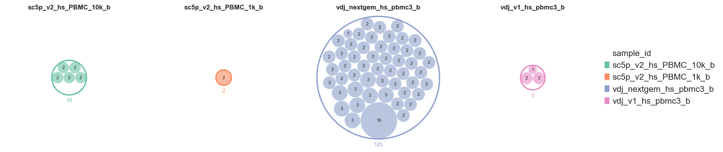
Setting as_subplots=True splits the figure into one panel per top-level group. scale_subplots=True (the default) scales enclosing circles proportionally to total cell count, so a clone of a given size always occupies the same area across panels.
[46]:
ddl.pl.clone_circlepackplot(
    vdj,
    group_by="sample_id",
    min_clone_size=2,
    as_subplots=True,
    show_count_labels=True,
    figsize=(4, 4),
)
plt.show()
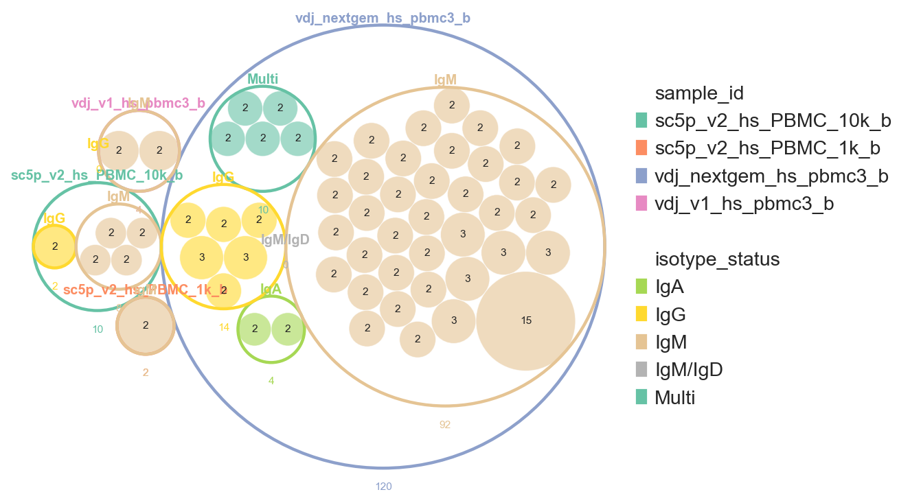
Passing a list to group_by produces a multi-level nesting. The hierarchy follows the list order: the first element is the outermost ring, subsequent elements are nested rings, and clone circles sit at the innermost level. Each level is coloured independently using its own colour map.
[47]:
ddl.pl.clone_circlepackplot(
    vdj,
    group_by=["sample_id", "isotype_status"],
    min_clone_size=2,
    show_count_labels=True,
    figsize=(7, 7),
)
plt.show()
min to max ratio is too low at 0.0 and it could cause algorithm stability issues. Try to remove insignificant data
min to max ratio is too low at 0.0 and it could cause algorithm stability issues. Try to remove insignificant data
Using different distance metrics in find_clones
By default, find_clones uses hamming distance as the distance metric, which only accounts for substitutions. If you want to account for insertions and deletions as well, you can change the distance metric to levenshtein or even BLOSUM62. You can also provide your own custom distance as a lambda function if you have specific requirements for how you want to define the distance between sequences. We will show you how to do this here:
[48]:
# let's reset vdj object to be lazy polars version
vdj.to_polars()
[49]:
# --- Levenshtein ---
vdj2 = vdj.copy()
adata2 = adata.copy()

ddl.tl.find_clones(
    vdj2, dist_func="levenshtein", same_vj=False, same_length=False
)
ddl.tl.generate_network(vdj2, use_existing_graph=False)
ddl.tl.transfer(adata2, vdj2)

ddl.pl.clone_network(
    adata2, color=["sample_id", "isotype_status"], edges_width=1, size=20
)
ddl.tl.clone_view(adata2, mode="expanded")
ddl.pl.clone_network(
    adata2, color=["sample_id", "isotype_status"], edges_width=1, size=20
)
Finding clonotypes
Finding clones based on B cell VDJ chains using junction_aa: 100%|██████████| 1/1 [00:00<00:00,  2.20it/s]
Finding clones based on B cell VJ chains using junction_aa: 100%|██████████| 1/1 [00:00<00:00,  5.76it/s]
Storing distance matrix...
Building distance matrix (batched): 100%|██████████| 1/1 [00:00<00:00, 1.78it/s]
Stored distances as CSR sparse matrix: (2353, 2353), density=99.32%
 finished: Updated Dandelion object:
   'data', contig AIRR table
   'metadata', cell observations table
   'distances', sparse distance matrix
 (0:00:01)
Generating network
Using pre-computed distances from .distances

Computing network layout
Computing expanded network layout
 finished.
   Updated Dandelion object
:    'layout', graph layout
 (0:00:00)
Transferring network
 finished: updated `.obs` with `.metadata`
wrote active layout to `.obsm['X_vdj']`; stashed all views in `.uns['dandelion']` ('X_vdj_all', 'X_vdj_expanded')
wrote `.obsp['connectivities']` & `['distances']` from graph[0]
stashed GEX matrices in `.uns['dandelion']` ('gex_connectivities', 'gex_distances')
stashed VDJ matrices in `.uns['dandelion']` under 'vdj_connectivities_all' / '_expanded'
added `.uns['clone_id']` clone-level mapping (0:00:00)
[50]:
# --- BLOSUM62 ---
# I'm not sure if this is working as intended because the resulting network looks very similar to the hamming distance one, but here is how you would do it:
vdj2 = vdj.copy()
adata2 = adata.copy()

ddl.tl.find_clones(vdj2, dist_func="blosum62", same_vj=False)
ddl.tl.generate_network(vdj2, use_existing_graph=False)
ddl.tl.transfer(adata2, vdj2)

ddl.pl.clone_network(
    adata2, color=["sample_id", "isotype_status"], edges_width=1, size=20
)
ddl.tl.clone_view(adata2, mode="expanded")
ddl.pl.clone_network(
    adata2, color=["sample_id", "isotype_status"], edges_width=1, size=20
)
Finding clonotypes
Finding clones based on B cell VDJ chains using junction_aa: 100%|██████████| 27/27 [00:00<00:00, 316.30it/s]
Finding clones based on B cell VJ chains using junction_aa: 100%|██████████| 14/14 [00:00<00:00, 132.14it/s]
Storing distance matrix...
Building distance matrix (batched): 100%|██████████| 1/1 [00:00<00:00, 13.87it/s]
Stored distances as CSR sparse matrix: (2353, 2353), density=36.43%
 finished: Updated Dandelion object:
   'data', contig AIRR table
   'metadata', cell observations table
   'distances', sparse distance matrix
 (0:00:00)
Generating network
Using pre-computed distances from .distances

Computing network layout
Computing expanded network layout
 finished.
   Updated Dandelion object
:    'layout', graph layout
 (0:00:00)
Transferring network
 finished: updated `.obs` with `.metadata`
wrote active layout to `.obsm['X_vdj']`; stashed all views in `.uns['dandelion']` ('X_vdj_all', 'X_vdj_expanded')
wrote `.obsp['connectivities']` & `['distances']` from graph[0]
stashed GEX matrices in `.uns['dandelion']` ('gex_connectivities', 'gex_distances')
stashed VDJ matrices in `.uns['dandelion']` under 'vdj_connectivities_all' / '_expanded'
added `.uns['clone_id']` clone-level mapping (0:00:00)
[51]:
# --- Custom lambda function ---
vdj2 = vdj.copy()
adata2 = adata.copy()

ddl.tl.find_clones(
    vdj2, dist_func=lambda x, y: 0 if x == y else 1
)  # this is basically a simple identity metric but with a custom function. You can make it as complex as you want as long as it takes in two sequences and outputs a distance metric.
ddl.tl.generate_network(vdj2, use_existing_graph=False)
ddl.tl.transfer(adata2, vdj2)

ddl.pl.clone_network(
    adata2, color=["sample_id", "isotype_status"], edges_width=1, size=20
)
ddl.tl.clone_view(adata2, mode="expanded")
ddl.pl.clone_network(
    adata2, color=["sample_id", "isotype_status"], edges_width=1, size=20
)
Finding clonotypes
Finding clones based on B cell VDJ chains using junction_aa: 100%|██████████| 1177/1177 [00:00<00:00, 15673.89it/s]
Finding clones based on B cell VJ chains using junction_aa: 100%|██████████| 485/485 [00:00<00:00, 11796.44it/s]
Storing distance matrix...
Building distance matrix (batched): 100%|██████████| 17/17 [00:00<00:00, 3684.54it/s]
Stored distances as CSR sparse matrix: (2353, 2353), density=0.72%
 finished: Updated Dandelion object:
   'data', contig AIRR table
   'metadata', cell observations table
   'distances', sparse distance matrix
 (0:00:00)
Generating network
Using pre-computed distances from .distances

Computing network layout
Computing expanded network layout
 finished.
   Updated Dandelion object
:    'layout', graph layout
 (0:00:00)
Transferring network
 finished: updated `.obs` with `.metadata`
wrote active layout to `.obsm['X_vdj']`; stashed all views in `.uns['dandelion']` ('X_vdj_all', 'X_vdj_expanded')
wrote `.obsp['connectivities']` & `['distances']` from graph[0]
stashed GEX matrices in `.uns['dandelion']` ('gex_connectivities', 'gex_distances')
stashed VDJ matrices in `.uns['dandelion']` under 'vdj_connectivities_all' / '_expanded'
added `.uns['clone_id']` clone-level mapping (0:00:00)