Calculating diversity and mutation
Calculating mutational load
To calculate mutational load, the functions from immcantation suite’s shazam [Gupta2015] can be accessed via rpy2 to work with the dandelion class object.
This can be run immediately after pp.reassign_alleles during the reannotation pre-processing stage because the required germline columns should be present in the genotyped .tsv file. I would recommend to run this after TIgGER [Gadala-Maria2015], after the v_calls were corrected. Otherwise, if the reannotation was skipped, you can run it now as follows:
Import modules
[1]:
import os
import dandelion as ddl
import matplotlib.pyplot as plt
import pandas as pd
import seaborn as sns
import scanpy as sc

sc.settings.verbosity = 3

ddl.set_backend("base")

# change to tutorials directory
os.chdir("dandelion_tutorial")
Read in the previously saved files
[2]:
adata = sc.read_h5ad("adata.h5ad")
adata
[2]:
AnnData object with n_obs × n_vars = 25063 × 1309
    obs: 'sample_id', 'n_genes', 'n_genes_by_counts', 'total_counts', 'total_counts_mt', 'pct_counts_mt', 'gmm_pct_count_clusters_keep', 'scrublet_score', 'is_doublet', 'filter_rna', 'has_contig', 'locus_VDJ', 'locus_VJ', 'productive_VDJ', 'productive_VJ', 'v_call_VDJ', 'd_call_VDJ', 'j_call_VDJ', 'v_call_VJ', 'j_call_VJ', 'c_call_VDJ', 'c_call_VJ', 'junction_VDJ', 'junction_VJ', 'junction_aa_VDJ', 'junction_aa_VJ', 'v_call_B_VDJ', 'd_call_B_VDJ', 'j_call_B_VDJ', 'v_call_B_VJ', 'j_call_B_VJ', 'c_call_B_VDJ', 'c_call_B_VJ', 'productive_B_VDJ', 'productive_B_VJ', 'umi_count_B_VDJ', 'umi_count_B_VJ', 'v_call_VDJ_main', 'v_call_VJ_main', 'd_call_VDJ_main', 'j_call_VDJ_main', 'j_call_VJ_main', 'c_call_VDJ_main', 'c_call_VJ_main', 'v_call_B_VDJ_main', 'd_call_B_VDJ_main', 'j_call_B_VDJ_main', 'v_call_B_VJ_main', 'j_call_B_VJ_main', 'isotype', 'isotype_status', 'locus_status', 'chain_status', 'rearrangement_status_VDJ', 'rearrangement_status_VJ', 'leiden', 'clone_id', 'clone_id_rank'
    var: 'n_cells', 'highly_variable', 'means', 'dispersions', 'dispersions_norm', 'mean', 'std'
    uns: 'chain_status_colors', 'clone_id', 'dandelion', 'gex_neighbors', 'hvg', 'isotype_status_colors', 'leiden', 'leiden_colors', 'locus_status_colors', 'log1p', 'neighbors', 'pca', 'sample_id_colors', 'umap'
    obsm: 'X_pca', 'X_umap', 'X_vdj'
    varm: 'PCs'
    obsp: 'connectivities', 'distances'
Note
This tutorial will be trying to quantify mutations in the BCR data, and this function requires access to IMGT-formatted VDJ gene calls with allelic information. So if you have ran vdj.simplify before this tutorial, then it would not work. Therefore, we are loading in the Dandelion object without simplified calls.
[3]:
vdj = ddl.read_h5ddl("dandelion_results.h5ddl")
vdj
[3]:
Dandelion class object with n_obs = 2496 and n_contigs = 7385
    data: 'sequence_id', 'sequence', 'rev_comp', 'productive', 'v_call', 'd_call', 'j_call', 'sequence_alignment', 'germline_alignment', 'junction', 'junction_aa', 'v_cigar', 'd_cigar', 'j_cigar', 'stop_codon', 'vj_in_frame', 'locus', 'c_call', 'junction_length', 'np1_length', 'np2_length', 'v_sequence_start', 'v_sequence_end', 'v_germline_start', 'v_germline_end', 'd_sequence_start', 'd_sequence_end', 'd_germline_start', 'd_germline_end', 'j_sequence_start', 'j_sequence_end', 'j_germline_start', 'j_germline_end', 'v_score', 'v_identity', 'v_support', 'd_score', 'd_identity', 'd_support', 'j_score', 'j_identity', 'j_support', 'fwr1', 'fwr2', 'fwr3', 'fwr4', 'cdr1', 'cdr2', 'cdr3', 'cell_id', 'consensus_count', 'umi_count', 'v_call_10x', 'd_call_10x', 'j_call_10x', 'junction_10x', 'junction_10x_aa', 'j_support_igblastn', 'j_score_igblastn', 'j_call_igblastn', 'j_call_blastn', 'j_identity_blastn', 'j_alignment_length_blastn', 'j_number_of_mismatches_blastn', 'j_number_of_gap_openings_blastn', 'j_sequence_start_blastn', 'j_sequence_end_blastn', 'j_germline_start_blastn', 'j_germline_end_blastn', 'j_support_blastn', 'j_score_blastn', 'j_sequence_alignment_blastn', 'j_germline_alignment_blastn', 'j_source', 'd_support_igblastn', 'd_score_igblastn', 'd_call_igblastn', 'd_call_blastn', 'd_identity_blastn', 'd_alignment_length_blastn', 'd_number_of_mismatches_blastn', 'd_number_of_gap_openings_blastn', 'd_sequence_start_blastn', 'd_sequence_end_blastn', 'd_germline_start_blastn', 'd_germline_end_blastn', 'd_support_blastn', 'd_score_blastn', 'd_sequence_alignment_blastn', 'd_germline_alignment_blastn', 'd_source', 'v_call_genotyped', 'germline_alignment_d_mask', 'sample_id', 'c_sequence_alignment', 'c_germline_alignment', 'c_sequence_start', 'c_sequence_end', 'c_score', 'c_identity', 'c_call_10x', 'junction_aa_length', 'fwr1_aa', 'fwr2_aa', 'fwr3_aa', 'fwr4_aa', 'cdr1_aa', 'cdr2_aa', 'cdr3_aa', 'sequence_alignment_aa', 'v_sequence_alignment_aa', 'd_sequence_alignment_aa', 'j_sequence_alignment_aa', 'complete_vdj', 'j_call_multimappers', 'j_call_multiplicity', 'j_call_sequence_start_multimappers', 'j_call_sequence_end_multimappers', 'j_call_support_multimappers', 'mu_count', 'rearrangement_status', 'v_call_functionality', 'd_call_functionality', 'j_call_functionality', 'ambiguous', 'extra'
    metadata: 'sample_id', 'locus_VDJ', 'locus_VJ', 'productive_VDJ', 'productive_VJ', 'v_call_VDJ', 'd_call_VDJ', 'j_call_VDJ', 'v_call_VJ', 'j_call_VJ', 'c_call_VDJ', 'c_call_VJ', 'junction_VDJ', 'junction_VJ', 'junction_aa_VDJ', 'junction_aa_VJ', 'v_call_B_VDJ', 'd_call_B_VDJ', 'j_call_B_VDJ', 'v_call_B_VJ', 'j_call_B_VJ', 'c_call_B_VDJ', 'c_call_B_VJ', 'productive_B_VDJ', 'productive_B_VJ', 'umi_count_B_VDJ', 'umi_count_B_VJ', 'v_call_VDJ_main', 'v_call_VJ_main', 'd_call_VDJ_main', 'j_call_VDJ_main', 'j_call_VJ_main', 'c_call_VDJ_main', 'c_call_VJ_main', 'v_call_B_VDJ_main', 'd_call_B_VDJ_main', 'j_call_B_VDJ_main', 'v_call_B_VJ_main', 'j_call_B_VJ_main', 'isotype', 'isotype_status', 'locus_status', 'chain_status', 'rearrangement_status_VDJ', 'rearrangement_status_VJ'
[4]:
# let's rerun the find_clone step again as it didn't get copied over
ddl.tl.find_clones(vdj)
Finding clonotypes
Finding clones based on B cell VDJ chains using junction_aa: 100%|██████████| 243/243 [00:00<00:00, 4083.28it/s]
Finding clones based on B cell VJ chains using junction_aa: 100%|██████████| 214/214 [00:00<00:00, 5270.93it/s]
Refining clone assignment based on VJ chain pairing : 100%|██████████| 2496/2496 [00:00<00:00, 659297.36it/s]
Initialising Dandelion object
 finished: Updated Dandelion object:
   'data', contig-indexed AIRR table
   'metadata', cell-indexed observations table
 (0:00:01)
[4]:
Dandelion class object with n_obs = 2496 and n_contigs = 7385
    data: 'sequence_id', 'sequence', 'rev_comp', 'productive', 'v_call', 'd_call', 'j_call', 'sequence_alignment', 'germline_alignment', 'junction', 'junction_aa', 'v_cigar', 'd_cigar', 'j_cigar', 'stop_codon', 'vj_in_frame', 'locus', 'c_call', 'junction_length', 'np1_length', 'np2_length', 'v_sequence_start', 'v_sequence_end', 'v_germline_start', 'v_germline_end', 'd_sequence_start', 'd_sequence_end', 'd_germline_start', 'd_germline_end', 'j_sequence_start', 'j_sequence_end', 'j_germline_start', 'j_germline_end', 'v_score', 'v_identity', 'v_support', 'd_score', 'd_identity', 'd_support', 'j_score', 'j_identity', 'j_support', 'fwr1', 'fwr2', 'fwr3', 'fwr4', 'cdr1', 'cdr2', 'cdr3', 'cell_id', 'consensus_count', 'umi_count', 'v_call_10x', 'd_call_10x', 'j_call_10x', 'junction_10x', 'junction_10x_aa', 'j_support_igblastn', 'j_score_igblastn', 'j_call_igblastn', 'j_call_blastn', 'j_identity_blastn', 'j_alignment_length_blastn', 'j_number_of_mismatches_blastn', 'j_number_of_gap_openings_blastn', 'j_sequence_start_blastn', 'j_sequence_end_blastn', 'j_germline_start_blastn', 'j_germline_end_blastn', 'j_support_blastn', 'j_score_blastn', 'j_sequence_alignment_blastn', 'j_germline_alignment_blastn', 'j_source', 'd_support_igblastn', 'd_score_igblastn', 'd_call_igblastn', 'd_call_blastn', 'd_identity_blastn', 'd_alignment_length_blastn', 'd_number_of_mismatches_blastn', 'd_number_of_gap_openings_blastn', 'd_sequence_start_blastn', 'd_sequence_end_blastn', 'd_germline_start_blastn', 'd_germline_end_blastn', 'd_support_blastn', 'd_score_blastn', 'd_sequence_alignment_blastn', 'd_germline_alignment_blastn', 'd_source', 'v_call_genotyped', 'germline_alignment_d_mask', 'sample_id', 'c_sequence_alignment', 'c_germline_alignment', 'c_sequence_start', 'c_sequence_end', 'c_score', 'c_identity', 'c_call_10x', 'junction_aa_length', 'fwr1_aa', 'fwr2_aa', 'fwr3_aa', 'fwr4_aa', 'cdr1_aa', 'cdr2_aa', 'cdr3_aa', 'sequence_alignment_aa', 'v_sequence_alignment_aa', 'd_sequence_alignment_aa', 'j_sequence_alignment_aa', 'complete_vdj', 'j_call_multimappers', 'j_call_multiplicity', 'j_call_sequence_start_multimappers', 'j_call_sequence_end_multimappers', 'j_call_support_multimappers', 'mu_count', 'rearrangement_status', 'v_call_functionality', 'd_call_functionality', 'j_call_functionality', 'ambiguous', 'extra', 'clone_id'
    metadata: 'clone_id', 'clone_id_rank', 'sample_id', 'locus_VDJ', 'locus_VJ', 'productive_VDJ', 'productive_VJ', 'v_call_VDJ', 'd_call_VDJ', 'j_call_VDJ', 'v_call_VJ', 'j_call_VJ', 'c_call_VDJ', 'c_call_VJ', 'junction_VDJ', 'junction_VJ', 'junction_aa_VDJ', 'junction_aa_VJ', 'v_call_B_VDJ', 'd_call_B_VDJ', 'j_call_B_VDJ', 'v_call_B_VJ', 'j_call_B_VJ', 'c_call_B_VDJ', 'c_call_B_VJ', 'productive_B_VDJ', 'productive_B_VJ', 'umi_count_B_VDJ', 'umi_count_B_VJ', 'v_call_VDJ_main', 'v_call_VJ_main', 'd_call_VDJ_main', 'j_call_VDJ_main', 'j_call_VJ_main', 'c_call_VDJ_main', 'c_call_VJ_main', 'v_call_B_VDJ_main', 'd_call_B_VDJ_main', 'j_call_B_VDJ_main', 'v_call_B_VJ_main', 'j_call_B_VJ_main', 'isotype', 'isotype_status', 'locus_status', 'chain_status', 'rearrangement_status_VDJ', 'rearrangement_status_VJ'
[5]:
# let's recreate the vdj object with only the first two samples
subset_data = vdj.data[
    vdj.data["sample_id"].isin(
        ["sc5p_v2_hs_PBMC_1k_b", "sc5p_v2_hs_PBMC_10k_b"]
    )
]
subset_data
[5]:
| sequence_id | sequence | rev_comp | productive | v_call | d_call | j_call | sequence_alignment | germline_alignment | junction | ... | j_call_sequence_end_multimappers | j_call_support_multimappers | mu_count | rearrangement_status | v_call_functionality | d_call_functionality | j_call_functionality | ambiguous | extra | clone_id | |
|---|---|---|---|---|---|---|---|---|---|---|---|---|---|---|---|---|---|---|---|---|---|
| sequence_id | |||||||||||||||||||||
| sc5p_v2_hs_PBMC_10k_b_AAACCTGTCATATCGG_contig_1 | sc5p_v2_hs_PBMC_10k_b_AAACCTGTCATATCGG_contig_1 | TGGGGAGGAGTCAGTCCCAACCAGGACACGGCCTGGACATGAGGGT... | F | T | IGKV1-33*01,IGKV1D-33*01 | IGKJ4*01 | GACATCCAGATGACCCAGTCTCCATCCTCCCTGTCTGCATCTGTGG... | GACATCCAGATGACCCAGTCTCCATCCTCCCTGTCTGCATCTGTAG... | TGTCAACAATATGACGAACTTCCCGTCACTTTC | ... | [412] | [3.56e-09] | 27 | standard | F | F | F | F | B_VJ_204_2_3 | ||
| sc5p_v2_hs_PBMC_10k_b_AAACCTGTCCGTTGTC_contig_2 | sc5p_v2_hs_PBMC_10k_b_AAACCTGTCCGTTGTC_contig_2 | ATCACATAACAACCACATTCCTCCTCTAAAGAAGCCCCTGGGAGCA... | F | T | IGHV1-69*01,IGHV1-69D*01 | IGHD3-22*01 | IGHJ3*02 | CAGGTGCAGCTGGTGCAGTCTGGGGCT...GAGGTGAAGAAGCCTG... | CAGGTGCAGCTGGTGCAGTCTGGGGCT...GAGGTGAAGAAGCCTG... | TGTGCGACTACGTATTACTATGATAGTAGTGGTTATTACCAGAATG... | ... | [494] | [4.5799999999999995e-23] | 0 | standard | F | F | F | F | F | B_VDJ_66_3_2_VJ_191_2_1 |
| sc5p_v2_hs_PBMC_10k_b_AAACCTGTCCGTTGTC_contig_1 | sc5p_v2_hs_PBMC_10k_b_AAACCTGTCCGTTGTC_contig_1 | AGGAGTCAGACCCTGTCAGGACACAGCATAGACATGAGGGTCCCCG... | F | T | IGKV1-8*01 | IGKJ1*01 | GCCATCCGGATGACCCAGTCTCCATCCTCATTCTCTGCATCTACAG... | GCCATCCGGATGACCCAGTCTCCATCCTCATTCTCTGCATCTACAG... | TGTCAACAGTATTATAGTTACCCTCGGACGTTC | ... | [415] | [2.7e-15] | 0 | standard | F | F | F | F | B_VDJ_66_3_2_VJ_191_2_1 | ||
| sc5p_v2_hs_PBMC_10k_b_AAACCTGTCGAGAACG_contig_1 | sc5p_v2_hs_PBMC_10k_b_AAACCTGTCGAGAACG_contig_1 | ACTGTGGGGGTAAGAGGTTGTGTCCACCATGGCCTGGACTCCTCTC... | F | T | IGLV5-45*02 | IGLJ3*02 | CAGGCTGTGCTGACTCAGCCGTCTTCC...CTCTCTGCATCTCCTG... | CAGGCTGTGCTGACTCAGCCGTCTTCC...CTCTCTGCATCTCCTG... | TGTATGATTTGGCACAGCAGCGCTTGGGTGGTC | ... | [431] | [6.84e-12] | 8 | standard | F | F | F | F | B_VDJ_147_1_2_VJ_176_1_1 | ||
| sc5p_v2_hs_PBMC_10k_b_AAACCTGTCGAGAACG_contig_2 | sc5p_v2_hs_PBMC_10k_b_AAACCTGTCGAGAACG_contig_2 | GGGAGCATCACCCAGCAACCACATCTGTCCTCTAGAGAATCCCCTG... | F | T | IGHV1-2*02 | IGHJ3*02 | CAGGTGCAACTGGTGCAGTCTGGGGGT...GAGGTAAAGAAGCCTG... | CAGGTGCAGCTGGTGCAGTCTGGGGCT...GAGGTGAAGAAGCCTG... | TGTGCGAGAGAGATAGAGGGGGACGGTGTTTTTGAAATCTGG | ... | [479] | [4.48e-18] | 22 | standard | F | F | F | F | B_VDJ_147_1_2_VJ_176_1_1 | ||
| ... | ... | ... | ... | ... | ... | ... | ... | ... | ... | ... | ... | ... | ... | ... | ... | ... | ... | ... | ... | ... | ... |
| sc5p_v2_hs_PBMC_1k_b_TTCCCAGAGTACATGA_contig_1 | sc5p_v2_hs_PBMC_1k_b_TTCCCAGAGTACATGA_contig_1 | AGGAATCAGACCCAGTCAGGACACAGCATGGACATGAGAGTCCTCG... | F | T | IGKV1-16*01 | IGKJ2*01,IGKJ2*02 | GACATCCAGATGACCCAGTCTCCATCCTCACTGTCTGCATCTGTGG... | GACATCCAGATGACCCAGTCTCCATCCTCACTGTCTGCATCTGTAG... | TGCCAACAATACATTACTGACCCGTTCACTTTT | ... | [412] | [4.56e-08] | 20 | standard | F | F | F | F | B_VDJ_231_10_15_VJ_26_1_4 | ||
| sc5p_v2_hs_PBMC_1k_b_TTGAACGCAGGCTGAA_contig_1 | sc5p_v2_hs_PBMC_1k_b_TTGAACGCAGGCTGAA_contig_1 | AGGAGTCAGACCCTGTCAGGACACAGCATAGACATGAGGGTCCCCG... | F | T | IGKV1-8*01 | IGKJ1*01 | GCCATCCGGATGACCCAGTCTCCATCCTCATTCTCTGCATCTACAG... | GCCATCCGGATGACCCAGTCTCCATCCTCATTCTCTGCATCTACAG... | TGTCAACAGTATTATAGTTACCCGTGGACGTTC | ... | [415] | [2.09e-16] | 0 | standard | F | F | F | F | B_VDJ_197_11_2_VJ_191_2_1 | ||
| sc5p_v2_hs_PBMC_1k_b_TTGAACGCAGGCTGAA_contig_2 | sc5p_v2_hs_PBMC_1k_b_TTGAACGCAGGCTGAA_contig_2 | CGAGCCCAGCACTGGAAGTCGCCGGTGTTTCCATTCGGTGATCATC... | F | T | IGHV3-30-3*01 | IGHD3-9*01 | IGHJ4*02 | CAGGTGCAGCTGGTGGAGTCTGGGGGA...GGCGTGGTCCAGCCTG... | CAGGTGCAGCTGGTGGAGTCTGGGGGA...GGCGTGGTCCAGCCTG... | TGTGCGAGAGATGAGTTAGATATTTTGACTGGTTACAATATCCCAA... | ... | [509] | [2.2e-16] | 0 | standard | F | F | F | F | F | B_VDJ_197_11_2_VJ_191_2_1 |
| sc5p_v2_hs_PBMC_1k_b_TTGCCGTAGAATGTGT_contig_1 | sc5p_v2_hs_PBMC_1k_b_TTGCCGTAGAATGTGT_contig_1 | GAGCTACAACAGGCAGGCAGGGGCAGCAAGATGGTGTTGCAGACCC... | F | T | IGKV4-1*01 | IGKJ2*01 | GACATCGTGATGACCCAGTCTCCAGACTCCCTGGCTGTGTCTCTGG... | GACATCGTGATGACCCAGTCTCCAGACTCCCTGGCTGTGTCTCTGG... | TGTCAGCAATATTATAGTACTCCGTACACTTTT | ... | [430] | [2.15e-16] | 0 | standard | F | F | F | F | B_VDJ_74_4_1_VJ_135_2_1 | ||
| sc5p_v2_hs_PBMC_1k_b_TTGCCGTAGAATGTGT_contig_2 | sc5p_v2_hs_PBMC_1k_b_TTGCCGTAGAATGTGT_contig_2 | TGGGGAGTGACTCCTGTGCCCCACCATGGACACACTTTGCTCCACG... | F | T | IGHV2-5*02 | IGHJ6*02 | CAGATCACCTTGAAGGAGTCTGGTCCT...ACGCTGGTGAAACCCA... | CAGATCACCTTGAAGGAGTCTGGTCCT...ACGCTGGTGAAACCCA... | TGTGCACACAGCGACTACTATGAGGGGCGCGGTATGGACGTCTGG | ... | [446] | [1.94e-21] | 0 | standard | F | F | F | F | B_VDJ_74_4_1_VJ_135_2_1 |
2579 rows × 127 columns
[6]:
# create a new Dandelion class with this subset
vdj2 = ddl.Dandelion(subset_data)
vdj2
The AIRR data needs to undergo sanitization, apologies for any delays...
[6]:
Dandelion class object with n_obs = 818 and n_contigs = 2579
    data: 'sequence_id', 'sequence', 'rev_comp', 'productive', 'v_call', 'd_call', 'j_call', 'sequence_alignment', 'germline_alignment', 'junction', 'junction_aa', 'v_cigar', 'd_cigar', 'j_cigar', 'stop_codon', 'vj_in_frame', 'locus', 'c_call', 'junction_length', 'np1_length', 'np2_length', 'v_sequence_start', 'v_sequence_end', 'v_germline_start', 'v_germline_end', 'd_sequence_start', 'd_sequence_end', 'd_germline_start', 'd_germline_end', 'j_sequence_start', 'j_sequence_end', 'j_germline_start', 'j_germline_end', 'v_score', 'v_identity', 'v_support', 'd_score', 'd_identity', 'd_support', 'j_score', 'j_identity', 'j_support', 'fwr1', 'fwr2', 'fwr3', 'fwr4', 'cdr1', 'cdr2', 'cdr3', 'cell_id', 'consensus_count', 'umi_count', 'v_call_10x', 'd_call_10x', 'j_call_10x', 'junction_10x', 'junction_10x_aa', 'j_support_igblastn', 'j_score_igblastn', 'j_call_igblastn', 'j_call_blastn', 'j_identity_blastn', 'j_alignment_length_blastn', 'j_number_of_mismatches_blastn', 'j_number_of_gap_openings_blastn', 'j_sequence_start_blastn', 'j_sequence_end_blastn', 'j_germline_start_blastn', 'j_germline_end_blastn', 'j_support_blastn', 'j_score_blastn', 'j_sequence_alignment_blastn', 'j_germline_alignment_blastn', 'j_source', 'd_support_igblastn', 'd_score_igblastn', 'd_call_igblastn', 'd_call_blastn', 'd_identity_blastn', 'd_alignment_length_blastn', 'd_number_of_mismatches_blastn', 'd_number_of_gap_openings_blastn', 'd_sequence_start_blastn', 'd_sequence_end_blastn', 'd_germline_start_blastn', 'd_germline_end_blastn', 'd_support_blastn', 'd_score_blastn', 'd_sequence_alignment_blastn', 'd_germline_alignment_blastn', 'd_source', 'v_call_genotyped', 'germline_alignment_d_mask', 'sample_id', 'c_sequence_alignment', 'c_germline_alignment', 'c_sequence_start', 'c_sequence_end', 'c_score', 'c_identity', 'c_call_10x', 'junction_aa_length', 'fwr1_aa', 'fwr2_aa', 'fwr3_aa', 'fwr4_aa', 'cdr1_aa', 'cdr2_aa', 'cdr3_aa', 'sequence_alignment_aa', 'v_sequence_alignment_aa', 'd_sequence_alignment_aa', 'j_sequence_alignment_aa', 'complete_vdj', 'j_call_multimappers', 'j_call_multiplicity', 'j_call_sequence_start_multimappers', 'j_call_sequence_end_multimappers', 'j_call_support_multimappers', 'mu_count', 'rearrangement_status', 'v_call_functionality', 'd_call_functionality', 'j_call_functionality', 'ambiguous', 'extra', 'clone_id'
    metadata: 'clone_id', 'clone_id_rank', 'sample_id', 'locus_VDJ', 'locus_VJ', 'productive_VDJ', 'productive_VJ', 'v_call_VDJ', 'd_call_VDJ', 'j_call_VDJ', 'v_call_VJ', 'j_call_VJ', 'c_call_VDJ', 'c_call_VJ', 'junction_VDJ', 'junction_VJ', 'junction_aa_VDJ', 'junction_aa_VJ', 'v_call_B_VDJ', 'd_call_B_VDJ', 'j_call_B_VDJ', 'v_call_B_VJ', 'j_call_B_VJ', 'c_call_B_VDJ', 'c_call_B_VJ', 'productive_B_VDJ', 'productive_B_VJ', 'umi_count_B_VDJ', 'umi_count_B_VJ', 'v_call_VDJ_main', 'v_call_VJ_main', 'd_call_VDJ_main', 'j_call_VDJ_main', 'j_call_VJ_main', 'c_call_VDJ_main', 'c_call_VJ_main', 'v_call_B_VDJ_main', 'd_call_B_VDJ_main', 'j_call_B_VDJ_main', 'v_call_B_VJ_main', 'j_call_B_VJ_main', 'isotype', 'isotype_status', 'locus_status', 'chain_status', 'rearrangement_status_VDJ', 'rearrangement_status_VJ'
store_germline_reference
We can store the corrected germline fasta files (after running TIgGER) in the Dandelion class as a dictionary.
[7]:
# update the germline using the corrected files after tigger
vdj2.store_germline_reference(
    corrected="tutorial_scgp1/tutorial_scgp1_heavy_igblast_db-pass_genotype.fasta",
    germline=None,
    org="human",
)
Updating germline reference
 finished: Updated Dandelion object:
   'germline', updated germline reference
 (0:00:00)
pp.create_germlines
Then we run pp.create_germline to (re)create the germline_alignment_d_mask column in the data. This works by calling CreateGermlines.py with only -d and -r options. Add further arguments with additional_args like below for your needs. See https://changeo.readthedocs.io/en/stable/examples/germlines.html for more info.
Note
In order for this function to work, the V/D/J calls need to be in IMGT format with allelic information. So if you have ran vdj.simplify before this step, then it would not work.
[8]:
ddl.pp.create_germlines(vdj2, additional_args=["--vf", "v_call_genotyped"])
Reconstructing germline sequences
Running command: CreateGermlines.py -d /private/var/folders/_r/j_8_fj3x28n2th3ch0ckn9c40000gt/T/tmpgc_w4q0u/tmp.tsv -r /var/folders/_r/j_8_fj3x28n2th3ch0ckn9c40000gt/T/tmpgc_w4q0u/germ.fasta --vf v_call_genotyped

     START> CreateGermlines
      FILE> tmp.tsv
GERM_TYPES> dmask
 SEQ_FIELD> sequence_alignment
   V_FIELD> v_call_genotyped
   D_FIELD> d_call
   J_FIELD> j_call
    CLONED> False

PROGRESS> 14:36:05 |####################| 100% (2,579) 0.0 min

 OUTPUT> tmp_germ-pass.tsv
RECORDS> 2579
   PASS> 2579
   FAIL> 0
    END> CreateGermlines

Updating germline reference
 finished: Updated Dandelion object:
   'germline', updated germline reference
 (0:00:00)
 finished: Returning Dandelion object:
 (0:00:02)
[8]:
Dandelion class object with n_obs = 818 and n_contigs = 2579
    data: 'sequence_id', 'sequence', 'rev_comp', 'productive', 'v_call', 'd_call', 'j_call', 'sequence_alignment', 'germline_alignment', 'junction', 'junction_aa', 'v_cigar', 'd_cigar', 'j_cigar', 'stop_codon', 'vj_in_frame', 'locus', 'c_call', 'junction_length', 'np1_length', 'np2_length', 'v_sequence_start', 'v_sequence_end', 'v_germline_start', 'v_germline_end', 'd_sequence_start', 'd_sequence_end', 'd_germline_start', 'd_germline_end', 'j_sequence_start', 'j_sequence_end', 'j_germline_start', 'j_germline_end', 'v_score', 'v_identity', 'v_support', 'd_score', 'd_identity', 'd_support', 'j_score', 'j_identity', 'j_support', 'fwr1', 'fwr2', 'fwr3', 'fwr4', 'cdr1', 'cdr2', 'cdr3', 'cell_id', 'consensus_count', 'umi_count', 'c_sequence_alignment', 'c_germline_alignment', 'c_sequence_start', 'c_sequence_end', 'c_score', 'c_identity', 'junction_aa_length', 'fwr1_aa', 'fwr2_aa', 'fwr3_aa', 'fwr4_aa', 'cdr1_aa', 'cdr2_aa', 'cdr3_aa', 'sequence_alignment_aa', 'v_sequence_alignment_aa', 'd_sequence_alignment_aa', 'j_sequence_alignment_aa', 'complete_vdj', 'clone_id', 'v_call_10x', 'd_call_10x', 'j_call_10x', 'junction_10x', 'junction_10x_aa', 'j_support_igblastn', 'j_score_igblastn', 'j_call_igblastn', 'j_call_blastn', 'j_identity_blastn', 'j_alignment_length_blastn', 'j_number_of_mismatches_blastn', 'j_number_of_gap_openings_blastn', 'j_sequence_start_blastn', 'j_sequence_end_blastn', 'j_germline_start_blastn', 'j_germline_end_blastn', 'j_support_blastn', 'j_score_blastn', 'j_sequence_alignment_blastn', 'j_germline_alignment_blastn', 'j_source', 'd_support_igblastn', 'd_score_igblastn', 'd_call_igblastn', 'd_call_blastn', 'd_identity_blastn', 'd_alignment_length_blastn', 'd_number_of_mismatches_blastn', 'd_number_of_gap_openings_blastn', 'd_sequence_start_blastn', 'd_sequence_end_blastn', 'd_germline_start_blastn', 'd_germline_end_blastn', 'd_support_blastn', 'd_score_blastn', 'd_sequence_alignment_blastn', 'd_germline_alignment_blastn', 'd_source', 'v_call_genotyped', 'germline_alignment_d_mask', 'sample_id', 'c_call_10x', 'j_call_multimappers', 'j_call_multiplicity', 'j_call_sequence_start_multimappers', 'j_call_sequence_end_multimappers', 'j_call_support_multimappers', 'mu_count', 'rearrangement_status', 'v_call_functionality', 'd_call_functionality', 'j_call_functionality', 'ambiguous', 'extra'
    metadata: 'clone_id', 'clone_id_rank', 'sample_id', 'locus_VDJ', 'locus_VJ', 'productive_VDJ', 'productive_VJ', 'v_call_VDJ', 'd_call_VDJ', 'j_call_VDJ', 'v_call_VJ', 'j_call_VJ', 'c_call_VDJ', 'c_call_VJ', 'junction_VDJ', 'junction_VJ', 'junction_aa_VDJ', 'junction_aa_VJ', 'v_call_B_VDJ', 'd_call_B_VDJ', 'j_call_B_VDJ', 'v_call_B_VJ', 'j_call_B_VJ', 'c_call_B_VDJ', 'c_call_B_VJ', 'productive_B_VDJ', 'productive_B_VJ', 'umi_count_B_VDJ', 'umi_count_B_VJ', 'v_call_VDJ_main', 'v_call_VJ_main', 'd_call_VDJ_main', 'j_call_VDJ_main', 'j_call_VJ_main', 'c_call_VDJ_main', 'c_call_VJ_main', 'v_call_B_VDJ_main', 'd_call_B_VDJ_main', 'j_call_B_VDJ_main', 'v_call_B_VJ_main', 'j_call_B_VJ_main', 'isotype', 'isotype_status', 'locus_status', 'chain_status', 'rearrangement_status_VDJ', 'rearrangement_status_VJ'
Ensure that the germline_alignment_d_mask column is populated or subsequent steps will fail.
[9]:
vdj2.data[["v_call_genotyped", "germline_alignment_d_mask"]]
[9]:
| v_call_genotyped | germline_alignment_d_mask | |
|---|---|---|
| sequence_id | ||
| sc5p_v2_hs_PBMC_10k_b_AAACCTGTCATATCGG_contig_1 | IGKV1-33*01,IGKV1D-33*01 | GACATCCAGATGACCCAGTCTCCATCCTCCCTGTCTGCATCTGTAG... |
| sc5p_v2_hs_PBMC_10k_b_AAACCTGTCCGTTGTC_contig_2 | IGHV1-69*01,IGHV1-69D*01 | CAGGTGCAGCTGGTGCAGTCTGGGGCT...GAGGTGAAGAAGCCTG... |
| sc5p_v2_hs_PBMC_10k_b_AAACCTGTCCGTTGTC_contig_1 | IGKV1-8*01 | GCCATCCGGATGACCCAGTCTCCATCCTCATTCTCTGCATCTACAG... |
| sc5p_v2_hs_PBMC_10k_b_AAACCTGTCGAGAACG_contig_1 | IGLV5-45*02 | CAGGCTGTGCTGACTCAGCCGTCTTCC...CTCTCTGCATCTCCTG... |
| sc5p_v2_hs_PBMC_10k_b_AAACCTGTCGAGAACG_contig_2 | IGHV1-2*02 | CAGGTGCAGCTGGTGCAGTCTGGGGCT...GAGGTGAAGAAGCCTG... |
| ... | ... | ... |
| sc5p_v2_hs_PBMC_1k_b_TTCCCAGAGTACATGA_contig_2 | IGHV3-23*01,IGHV3-23D*01 | GAGGTGCAGCTGTTGGAGTCTGGGGGA...GGCTTGGTACAGCCTG... |
| sc5p_v2_hs_PBMC_1k_b_TTGAACGCAGGCTGAA_contig_1 | IGKV1-8*01 | GCCATCCGGATGACCCAGTCTCCATCCTCATTCTCTGCATCTACAG... |
| sc5p_v2_hs_PBMC_1k_b_TTGAACGCAGGCTGAA_contig_2 | IGHV3-30-3*01 | CAGGTGCAGCTGGTGGAGTCTGGGGGA...GGCGTGGTCCAGCCTG... |
| sc5p_v2_hs_PBMC_1k_b_TTGCCGTAGAATGTGT_contig_1 | IGKV4-1*01 | GACATCGTGATGACCCAGTCTCCAGACTCCCTGGCTGTGTCTCTGG... |
| sc5p_v2_hs_PBMC_1k_b_TTGCCGTAGAATGTGT_contig_2 | IGHV2-5*02 | CAGATCACCTTGAAGGAGTCTGGTCCT...ACGCTGGTGAAACCCA... |
2579 rows × 2 columns
The default behaviour is to mask the D region with Ns with option.
pp.quantify_mutations
The options for pp.quantify_mutations are the same as the basic mutational load analysis vignette [Gupta2015]. The default behavior is to sum all mutations scores (heavy and light chains, silent and replacement mutations) for the same cell.
Again, this function can be run immediately after pp.reassign_alleles on the genotyped .tsv files (without loading into pandas or Dandelion). Here I’m illustrating a few other options that may be useful.
[10]:
# switching back to using the full vdj object
ddl.pp.quantify_mutations(vdj)
Quantifying mutations
 finished: Updated Dandelion object:
   'data', contig-indexed AIRR table
   'metadata', cell-indexed observations table
 (0:00:15)
[11]:
ddl.pp.quantify_mutations(vdj, combine=False)
Quantifying mutations
 finished: Updated Dandelion object:
   'data', contig-indexed AIRR table
   'metadata', cell-indexed observations table
 (0:00:08)
Specifying split_locus = True will split up the results for the different chains.
[12]:
ddl.pp.quantify_mutations(vdj, split_locus=True)
Quantifying mutations
 finished: Updated Dandelion object:
   'data', contig-indexed AIRR table
   'metadata', cell-indexed observations table
 (0:00:09)
To update the AnnData object, simply rerun tl.transfer.
[13]:
ddl.tl.transfer(adata, vdj)
Transferring network
 finished: updated `.obs` with `.metadata`
 (0:00:00)
[14]:
adata
[14]:
AnnData object with n_obs × n_vars = 25063 × 1309
    obs: 'sample_id', 'n_genes', 'n_genes_by_counts', 'total_counts', 'total_counts_mt', 'pct_counts_mt', 'gmm_pct_count_clusters_keep', 'scrublet_score', 'is_doublet', 'filter_rna', 'has_contig', 'locus_VDJ', 'locus_VJ', 'productive_VDJ', 'productive_VJ', 'v_call_VDJ', 'd_call_VDJ', 'j_call_VDJ', 'v_call_VJ', 'j_call_VJ', 'c_call_VDJ', 'c_call_VJ', 'junction_VDJ', 'junction_VJ', 'junction_aa_VDJ', 'junction_aa_VJ', 'v_call_B_VDJ', 'd_call_B_VDJ', 'j_call_B_VDJ', 'v_call_B_VJ', 'j_call_B_VJ', 'c_call_B_VDJ', 'c_call_B_VJ', 'productive_B_VDJ', 'productive_B_VJ', 'umi_count_B_VDJ', 'umi_count_B_VJ', 'v_call_VDJ_main', 'v_call_VJ_main', 'd_call_VDJ_main', 'j_call_VDJ_main', 'j_call_VJ_main', 'c_call_VDJ_main', 'c_call_VJ_main', 'v_call_B_VDJ_main', 'd_call_B_VDJ_main', 'j_call_B_VDJ_main', 'v_call_B_VJ_main', 'j_call_B_VJ_main', 'isotype', 'isotype_status', 'locus_status', 'chain_status', 'rearrangement_status_VDJ', 'rearrangement_status_VJ', 'leiden', 'clone_id', 'clone_id_rank', 'mu_count', 'mu_count_seq_r', 'mu_count_seq_s', 'mu_count_seq_r_IGL', 'mu_count_seq_s_IGL', 'mu_count_IGL', 'mu_count_seq_r_IGK', 'mu_count_seq_s_IGK', 'mu_count_IGK', 'mu_count_seq_r_IGH', 'mu_count_seq_s_IGH', 'mu_count_IGH'
    var: 'n_cells', 'highly_variable', 'means', 'dispersions', 'dispersions_norm', 'mean', 'std'
    uns: 'chain_status_colors', 'clone_id', 'dandelion', 'gex_neighbors', 'hvg', 'isotype_status_colors', 'leiden', 'leiden_colors', 'locus_status_colors', 'log1p', 'neighbors', 'pca', 'sample_id_colors', 'umap'
    obsm: 'X_pca', 'X_umap', 'X_vdj'
    varm: 'PCs'
    obsp: 'connectivities', 'distances'
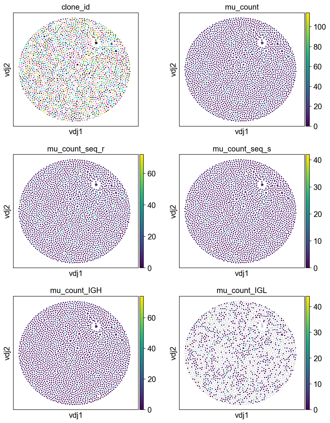
[15]:
from scanpy.plotting.palettes import default_28, default_102

sc.set_figure_params(figsize=[4, 4])
ddl.pl.clone_network(
    adata,
    color=[
        "clone_id",
        "mu_count",
        "mu_count_seq_r",
        "mu_count_seq_s",
        "mu_count_IGH",
        "mu_count_IGL",
    ],
    ncols=2,
    legend_loc="none",
    legend_fontoutline=3,
    edges_width=1,
    palette=default_28 + default_102,
    color_map="viridis",
    size=20,
)
WARNING: Length of palette colors is smaller than the number of categories (palette length: 130, categories length: 2257. Some categories will have the same color.
Calculating diversity
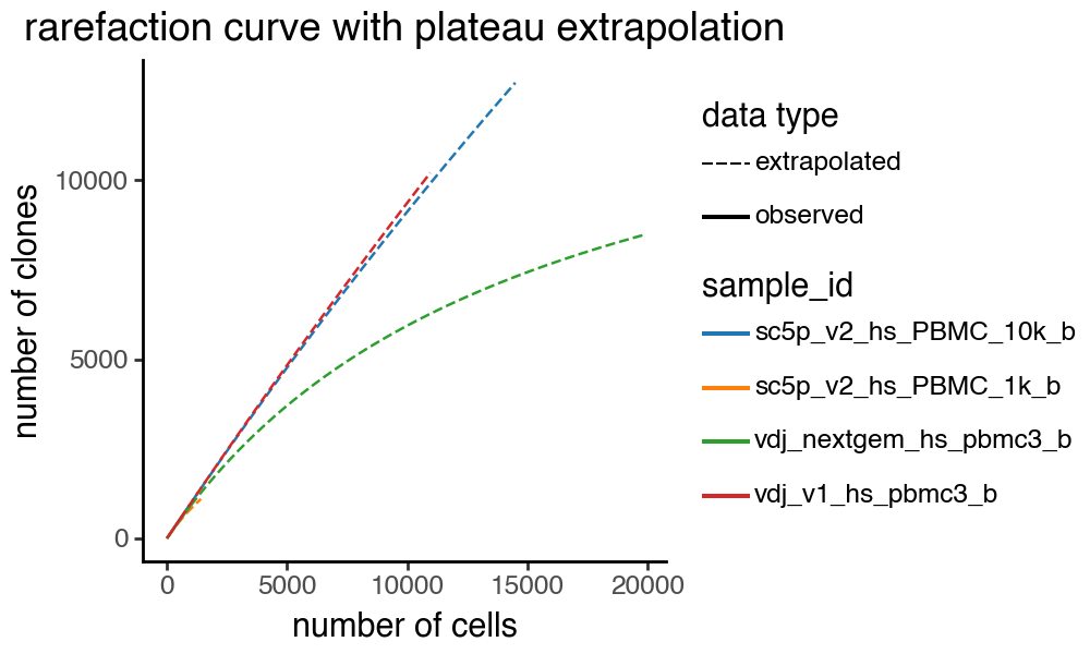
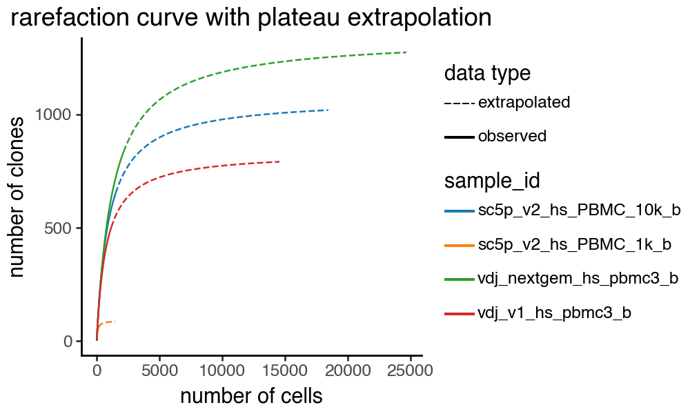
ddl.tl.clone_rarefaction
We can use ddl.tl.clone_rarefaction to generate rarefaction curves for the clones. Here, I am grouping by sampleid in the AnnData object. The function will work on both AnnData and Dandelion objects. We fit the rarefaction curves using a Michaelis–Menten model and extrapolate them beyond the observed data points, with the asymptote providing an estimate of the expected number of unique clones at larger sample sizes.
[16]:
ddl.tl.clone_rarefaction(adata, group_by="sample_id", plot=True)
Calculating rarefaction + extrapolation: 100%|██████████| 4/4 [00:00<00:00, 8.47it/s]
You can also use it to return the results without plotting:
[17]:
pred = ddl.tl.clone_rarefaction(adata, group_by="sample_id", plot=False)
pred
Calculating rarefaction + extrapolation: 100%|██████████| 4/4 [00:00<00:00, 7.83it/s]
[17]:
| cells | yhat | group | type | plateau | |
|---|---|---|---|---|---|
| 0 | 1 | 0.986026 | vdj_nextgem_hs_pbmc3_b | observed | 14283.506234 |
| 1 | 2 | 1.971922 | vdj_nextgem_hs_pbmc3_b | observed | 14283.506234 |
| 2 | 3 | 2.957689 | vdj_nextgem_hs_pbmc3_b | observed | 14283.506234 |
| 3 | 4 | 3.943327 | vdj_nextgem_hs_pbmc3_b | observed | 14283.506234 |
| 4 | 5 | 4.928836 | vdj_nextgem_hs_pbmc3_b | observed | 14283.506234 |
| ... | ... | ... | ... | ... | ... |
| 46771 | 1415 | 1096.798517 | sc5p_v2_hs_PBMC_1k_b | extrapolated | 4628.762094 |
| 46772 | 1416 | 1097.399060 | sc5p_v2_hs_PBMC_1k_b | extrapolated | 4628.762094 |
| 46773 | 1417 | 1097.999412 | sc5p_v2_hs_PBMC_1k_b | extrapolated | 4628.762094 |
| 46774 | 1418 | 1098.599573 | sc5p_v2_hs_PBMC_1k_b | extrapolated | 4628.762094 |
| 46775 | 1419 | 1099.199543 | sc5p_v2_hs_PBMC_1k_b | extrapolated | 4628.762094 |
46776 rows × 5 columns
Let’s try and resample the data to a larger number of cells to see how many unique clones we would expect to see if we simulated to have more data.
[18]:
vdj_large = ddl.tl.vdj_sample(vdj_data=vdj, size=5000)
# re-run clone finding on the larger dataset
ddl.tl.find_clones(vdj_large)
ddl.tl.clone_rarefaction(
    vdj_large,
    group_by="sample_id",
    plot=True,
    palette=adata.uns["sample_id_colors"],
)
Resampling to 5000 cells.
The AIRR data needs to undergo sanitization, apologies for any delays...
Finding clonotypes
Finding clones based on B cell VDJ chains using junction_aa: 100%|██████████| 234/234 [00:00<00:00, 5081.87it/s]
Finding clones based on B cell VJ chains using junction_aa: 100%|██████████| 205/205 [00:00<00:00, 5336.00it/s]
Refining clone assignment based on VJ chain pairing : 100%|██████████| 5000/5000 [00:00<00:00, 600369.87it/s]
Initialising Dandelion object
 finished: Updated Dandelion object:
   'data', contig-indexed AIRR table
   'metadata', cell-indexed observations table
 (0:00:03)
Calculating rarefaction + extrapolation: 100%|██████████| 4/4 [00:00<00:00, 5.83it/s]
ddl.tl.clone_diversity
ddl.tl.clone_diversity allows for calculation of diversity measures such as Chao1, Shannon Entropy and Gini indices.
For Gini indices, we provide several types of measures, inspired by bulk BCRseq analysis methods from [Bashford-Rogers2013]:
The following two indices are returned with network_metric="clone_network".
network cluster/clone size Gini index
In a contracted BCR network (where identical BCRs are collapsed into the same node/vertex), disparity in the distribution should be correlated to the amount of mutation events i.e. larger networks should indicate more mutation events and smaller networks should indicate lesser mutation events.
network vertex/node size Gini index
In the same contracted network, we can count the number of merged/contracted nodes; nodes with higher count numbers indicate more clonal expansion. Thus, disparity in the distribution of count numbers (referred to as vertex size) should be correlated to the overall clonality i.e. clones with larger vertex sizes are more monoclonal and clones with smaller vertex sizes are more polyclonal.
Therefore, a Gini index of 1 on either measures repesents perfect inequality (i.e. monoclonal and highly mutated) and a value of 0 represents perfect equality (i.e. polyclonal and unmutated).
Note
However, there are a few limitations/challenges that comes with single-cell data:
In the process of contracting the network, we discard the single-cell level information.
Contraction of network is very slow, particularly when there is a lot of clonally-related cells.
For the full implementation and interpretation of both measures, although more evident with cluster/clone size, it requires the BCR repertoire to be reasonably/deeply sampled and we know that this is currently limited by the low recovery from single cell data with current technologies.
Therefore, we implement a few work around options, and ‘experimental’ options below, to try and circumvent these issues.
Firstly, as a work around for (C), the cluster size gini index can be calculated before or after network contraction. If performing before network contraction (default), it will be calculated based on the size of subgraphs of connected components in the main graph. This will retain the single-cell information and should appropriately show the distribution of the data. If performing after network contraction, the calculation is performed after network contraction, achieving the same effect as the
method for bulk BCR-seq as described above. This option can be toggled by use_contracted and only applies to network cluster size gini index calculation.
clone centrality Gini index -
network_metric="clone_centrality"
Node/vertex closeness centrality indicates how tightly packed clones are (more clonally related) and thus the distribution of the number of cells connected in each clone informs on whether clones in general are more monoclonal or polyclonal.
clone degree Gini index -
network_metric="clone_degree"
Node/vertex degree indicates how many cells are connected to an individual cell, another indication of how clonally related cells are. However, this would also highlight cells that are in the middle of large networks but are not necessarily within clonally expanded regions (e.g. intermediate connecting cells within the minimum spanning tree).
clone size Gini index -
network_metric="clone_size"
This is not to be confused with the network cluster size gini index calculation above as this doesn’t rely on the network, although the values should be similar. This is just a simple implementation based on the data frame for the relevant clone_id column. By default, this metric is also returned when running network_metric=clone_centrality or network_metric=clone_degree.
Note
For (I) and (II), we can specify expanded_only option to compute the statistic for all clones or expanded only clones. Unlike options (I) and (II), the current calculation for (III) and (IV) is largely influenced by the amount of expanded clones i.e. clones with at least 2 cells, and not affected by the number of singleton clones because singleton clones will have a value of 0 regardless.
All the diversity functions will perform bootstrap sampling with replacements to estimate confidence intervals.
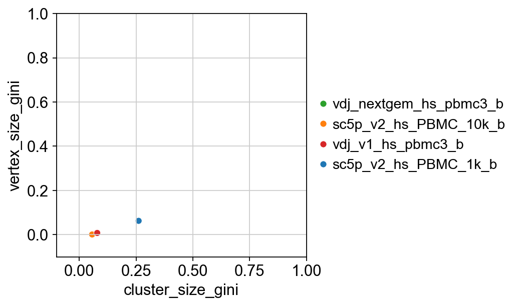
[19]:
results, raw = ddl.tl.clone_diversity(
    vdj,
    group_by="sample_id",
    method="gini",
    network_metric="clone_network",
    n_boot=200,
    n_cpus=8,
    verbose=True,
)
results
Calculating Gini indices
Bootstrapping... vdj_nextgem_hs_pbmc3_b: 100%|██████████| 200/200 [00:25<00:00,  7.81it/s]
Bootstrapping... sc5p_v2_hs_PBMC_10k_b: 100%|██████████| 200/200 [00:17<00:00, 11.73it/s]
Bootstrapping... vdj_v1_hs_pbmc3_b: 100%|██████████| 200/200 [00:16<00:00, 12.16it/s]
Bootstrapping... sc5p_v2_hs_PBMC_1k_b: 100%|██████████| 200/200 [00:15<00:00, 13.32it/s]
[19]:
{'cluster_size_gini':                 sample_id      mean       std  lower_95  upper_95
 0  vdj_nextgem_hs_pbmc3_b  0.081477  0.025944  0.040145  0.134633
 1   sc5p_v2_hs_PBMC_10k_b  0.057245  0.022155  0.027022  0.099366
 2       vdj_v1_hs_pbmc3_b  0.074761  0.023559  0.027022  0.123140
 3    sc5p_v2_hs_PBMC_1k_b  0.263552  0.021332  0.222216  0.306274,
 'vertex_size_gini':                 sample_id      mean       std  lower_95  upper_95
 0  vdj_nextgem_hs_pbmc3_b  0.007224  0.006300  0.000000  0.019435
 1   sc5p_v2_hs_PBMC_10k_b  0.001478  0.004248  0.000000  0.010474
 2       vdj_v1_hs_pbmc3_b  0.006604  0.008988  0.000000  0.027426
 3    sc5p_v2_hs_PBMC_1k_b  0.065373  0.018857  0.034581  0.101708}
[20]:
# let's merge the two results dataframes for easier plotting
cluster_size = results["cluster_size_gini"][["sample_id", "mean"]]
vertex_size = results["vertex_size_gini"][["sample_id", "mean"]]
cluster_size.rename(columns={"mean": "cluster_size_gini"}, inplace=True)
vertex_size.rename(columns={"mean": "vertex_size_gini"}, inplace=True)
combined_results = pd.concat(
    [cluster_size.set_index("sample_id"), vertex_size.set_index("sample_id")],
    axis=1,
)
# set the colours
palette = dict(
    zip(adata.obs["sample_id"].cat.categories, adata.uns["sample_id_colors"])
)
p = sns.scatterplot(
    x="cluster_size_gini",
    y="vertex_size_gini",
    data=combined_results,
    hue=combined_results.index,
    palette=palette,
)
p.set(ylim=(-0.1, 1), xlim=(-0.1, 1))
plt.legend(bbox_to_anchor=(1, 0.5), loc="center left", frameon=False)
plt.show()
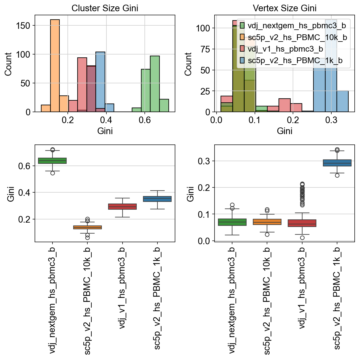
We can also plot the raw bootstrapped distributions for each sample to visualise the spread of the values.
[21]:
fig, axes = plt.subplots(2, 2, figsize=(8, 8))  # 1 row, 2 columns
sns.histplot(
    data=raw["cluster_size_gini"],
    palette=palette,
    ax=axes[0, 0],
)
sns.histplot(
    data=raw["vertex_size_gini"],
    palette=palette,
    ax=axes[0, 1],
)
sns.boxplot(
    data=raw["cluster_size_gini"],
    palette=palette,
    ax=axes[1, 0],
)
sns.boxplot(
    data=raw["vertex_size_gini"],
    palette=palette,
    ax=axes[1, 1],
)
axes[0, 0].set_title("Cluster Size Gini")
axes[0, 1].set_title("Vertex Size Gini")
axes[0, 0].legend_.remove()
axes[0, 0].set_xlabel("Gini")
axes[0, 1].set_xlabel("Gini")
axes[1, 0].set_ylabel("Gini")
axes[1, 1].set_ylabel("Gini")
axes[1, 0].set_xticklabels(axes[1, 0].get_xticklabels(), rotation=90)
axes[1, 1].set_xticklabels(axes[1, 1].get_xticklabels(), rotation=90)
plt.tight_layout()
plt.show()
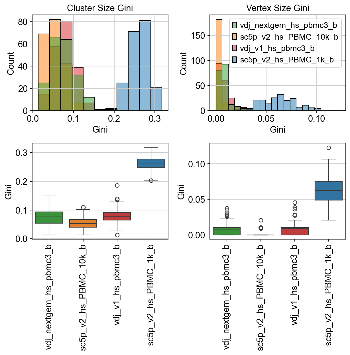
With these particular samples, because there is not many expanded clones in general, the gini indices are quite low when calculated within each sample. Let’s try and simulate a really large number of cells.
[22]:
# now let's create a large sample using vdj_sample with probability weighting based on the clone size proportions so that larger clones are more likely to be sampled
ddl.tl.clone_size(vdj)
vdj_large = ddl.tl.vdj_sample(
    vdj_data=vdj,
    size=10000,
    p=vdj.metadata["clone_id_size_prop"],
    random_state=42,
)
vdj_large
Resampling to 10000 cells.
The AIRR data needs to undergo sanitization, apologies for any delays...
[22]:
Dandelion class object with n_obs = 10000 and n_contigs = 16046
    data: 'sequence_id', 'sequence', 'rev_comp', 'productive', 'v_call', 'd_call', 'j_call', 'sequence_alignment', 'germline_alignment', 'junction', 'junction_aa', 'v_cigar', 'd_cigar', 'j_cigar', 'stop_codon', 'vj_in_frame', 'locus', 'c_call', 'junction_length', 'np1_length', 'np2_length', 'v_sequence_start', 'v_sequence_end', 'v_germline_start', 'v_germline_end', 'd_sequence_start', 'd_sequence_end', 'd_germline_start', 'd_germline_end', 'j_sequence_start', 'j_sequence_end', 'j_germline_start', 'j_germline_end', 'v_score', 'v_identity', 'v_support', 'd_score', 'd_identity', 'd_support', 'j_score', 'j_identity', 'j_support', 'fwr1', 'fwr2', 'fwr3', 'fwr4', 'cdr1', 'cdr2', 'cdr3', 'cell_id', 'consensus_count', 'umi_count', 'v_call_10x', 'd_call_10x', 'j_call_10x', 'junction_10x', 'junction_10x_aa', 'j_support_igblastn', 'j_score_igblastn', 'j_call_igblastn', 'j_call_blastn', 'j_identity_blastn', 'j_alignment_length_blastn', 'j_number_of_mismatches_blastn', 'j_number_of_gap_openings_blastn', 'j_sequence_start_blastn', 'j_sequence_end_blastn', 'j_germline_start_blastn', 'j_germline_end_blastn', 'j_support_blastn', 'j_score_blastn', 'j_sequence_alignment_blastn', 'j_germline_alignment_blastn', 'j_source', 'd_support_igblastn', 'd_score_igblastn', 'd_call_igblastn', 'd_call_blastn', 'd_identity_blastn', 'd_alignment_length_blastn', 'd_number_of_mismatches_blastn', 'd_number_of_gap_openings_blastn', 'd_sequence_start_blastn', 'd_sequence_end_blastn', 'd_germline_start_blastn', 'd_germline_end_blastn', 'd_support_blastn', 'd_score_blastn', 'd_sequence_alignment_blastn', 'd_germline_alignment_blastn', 'd_source', 'v_call_genotyped', 'germline_alignment_d_mask', 'sample_id', 'c_sequence_alignment', 'c_germline_alignment', 'c_sequence_start', 'c_sequence_end', 'c_score', 'c_identity', 'c_call_10x', 'junction_aa_length', 'fwr1_aa', 'fwr2_aa', 'fwr3_aa', 'fwr4_aa', 'cdr1_aa', 'cdr2_aa', 'cdr3_aa', 'sequence_alignment_aa', 'v_sequence_alignment_aa', 'd_sequence_alignment_aa', 'j_sequence_alignment_aa', 'complete_vdj', 'j_call_multimappers', 'j_call_multiplicity', 'j_call_sequence_start_multimappers', 'j_call_sequence_end_multimappers', 'j_call_support_multimappers', 'mu_count', 'rearrangement_status', 'v_call_functionality', 'd_call_functionality', 'j_call_functionality', 'ambiguous', 'extra', 'clone_id', 'mu_count_seq_r', 'mu_count_seq_s'
    metadata: 'clone_id', 'clone_id_rank', 'sample_id', 'locus_VDJ', 'locus_VJ', 'productive_VDJ', 'productive_VJ', 'v_call_VDJ', 'd_call_VDJ', 'j_call_VDJ', 'v_call_VJ', 'j_call_VJ', 'c_call_VDJ', 'c_call_VJ', 'junction_VDJ', 'junction_VJ', 'junction_aa_VDJ', 'junction_aa_VJ', 'v_call_B_VDJ', 'd_call_B_VDJ', 'j_call_B_VDJ', 'v_call_B_VJ', 'j_call_B_VJ', 'c_call_B_VDJ', 'c_call_B_VJ', 'productive_B_VDJ', 'productive_B_VJ', 'umi_count_B_VDJ', 'umi_count_B_VJ', 'v_call_VDJ_main', 'v_call_VJ_main', 'd_call_VDJ_main', 'j_call_VDJ_main', 'j_call_VJ_main', 'c_call_VDJ_main', 'c_call_VJ_main', 'v_call_B_VDJ_main', 'd_call_B_VDJ_main', 'j_call_B_VDJ_main', 'v_call_B_VJ_main', 'j_call_B_VJ_main', 'isotype', 'isotype_status', 'locus_status', 'chain_status', 'rearrangement_status_VDJ', 'rearrangement_status_VJ'
Let’s also go a bit further and introduce some mutations into the sequences to see how that affects the diversity measures.
[23]:
from Bio.Seq import Seq
import random

NUCLEOTIDES = ["A", "T", "C", "G"]
GAP_CHARS = {".", "-", "N"}  # You can extend this set if needed


def mutate_sequence(seq, mutation_rate=0.01):
    """Randomly mutate nucleotide sequence but skip gap characters."""
    seq_list = list(seq)

    for i, nt in enumerate(seq_list):
        # Skip gaps or unknown characters
        if nt.upper() not in NUCLEOTIDES:
            continue

        if random.random() < mutation_rate:
            # choose any nucleotide except the current one
            seq_list[i] = random.choice(
                [n for n in NUCLEOTIDES if n != nt.upper()]
            )

    return "".join(seq_list)


def translate_cleaned_nt(seq):
    """Remove gap characters and translate clean nucleotide sequence."""
    cleaned = "".join([nt for nt in seq if nt.upper() in NUCLEOTIDES])
    return str(Seq(cleaned).translate(to_stop=False))


def mutate_dataframe(df, nt_col="junction", mutation_rate=0.01):
    """Mutate nucleotide sequences in the DataFrame and update amino acids."""
    mutated_nt = []
    mutated_aa = []
    aa_col = nt_col + "_aa"
    for nt_seq in df[nt_col]:
        mutated_seq = mutate_sequence(nt_seq, mutation_rate)
        mutated_nt.append(mutated_seq)

        aa_seq = translate_cleaned_nt(mutated_seq)
        mutated_aa.append(aa_seq)

    df[nt_col] = mutated_nt
    df[aa_col] = mutated_aa
    return df
[24]:
vdj_large.data = mutate_dataframe(
    vdj_large.data, nt_col="sequence_alignment", mutation_rate=0.01
)
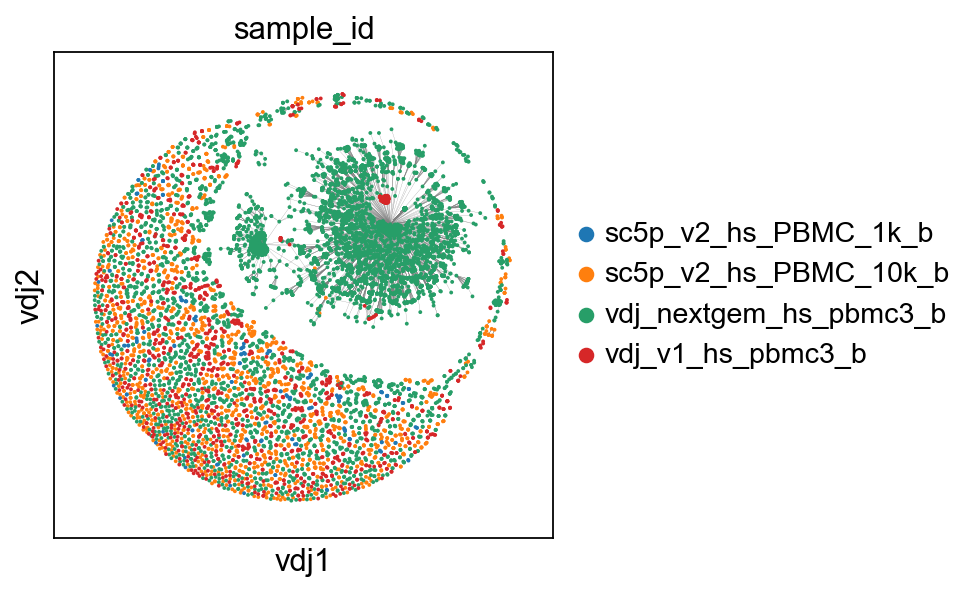
[25]:
# what does this dataset look like?
# Beware that this part is computationally intensive as we have a large dataset with many clones and sequences on the base backend. Should be fairly fast in polars though!
ddl.tl.generate_network(vdj_large, use_existing_graph=False)
adata_large = sc.AnnData(obs=vdj_large.metadata)
ddl.tl.transfer(adata_large, vdj_large)
ddl.pl.clone_network(adata_large, color=["sample_id"])
Generating network
Setting up data: 16046it [00:01, 8095.14it/s]
Calculating distance matrix with distance_mode = 'clone'
100%|██████████| 2280/2280 [04:32<00:00, 8.36it/s]
Distances calculated in 272.85 seconds
Sorting into clusters : 100%|██████████| 2280/2280 [00:01<00:00, 2230.50it/s]
Calculating minimum spanning tree : 100%|██████████| 1440/1440 [00:33<00:00, 42.46it/s]
Generating edge list : 100%|██████████| 1440/1440 [00:00<00:00, 4656.97it/s]
Computing overlap : 100%|██████████| 2280/2280 [00:02<00:00, 1092.22it/s]
Adjust overlap : 100%|██████████| 146/146 [00:00<00:00, 2189.10it/s]
Linking edges : 100%|██████████| 2043/2043 [03:56<00:00,  8.63it/s]
Computing network layout
Computing expanded network layout
 finished.
   Updated Dandelion object
:    'layout', graph layout
 (0:18:11)
Transferring network
 finished: updated `.obs` with `.metadata`
wrote active layout to `.obsm['X_vdj']`; stashed all views in `.uns['dandelion']` ('X_vdj_all', 'X_vdj_expanded')
wrote `.obsp['connectivities']` & `['distances']` from graph[0]
stashed VDJ matrices in `.uns['dandelion']` under 'vdj_connectivities_*' keys
added `.uns['clone_id']` clone-level mapping (0:00:04)
[26]:
results, raw = ddl.tl.clone_diversity(
    vdj_large,
    group_by="sample_id",
    method="gini",
    network_metric="clone_network",
    n_boot=200,
    n_cpus=8,
    verbose=True,
)
results
Calculating Gini indices
Bootstrapping... vdj_nextgem_hs_pbmc3_b: 100%|██████████| 200/200 [01:05<00:00,  3.04it/s]
Bootstrapping... sc5p_v2_hs_PBMC_10k_b: 100%|██████████| 200/200 [00:39<00:00,  5.04it/s]
Bootstrapping... vdj_v1_hs_pbmc3_b: 100%|██████████| 200/200 [00:35<00:00,  5.70it/s]
Bootstrapping... sc5p_v2_hs_PBMC_1k_b: 100%|██████████| 200/200 [00:30<00:00,  6.58it/s]
[26]:
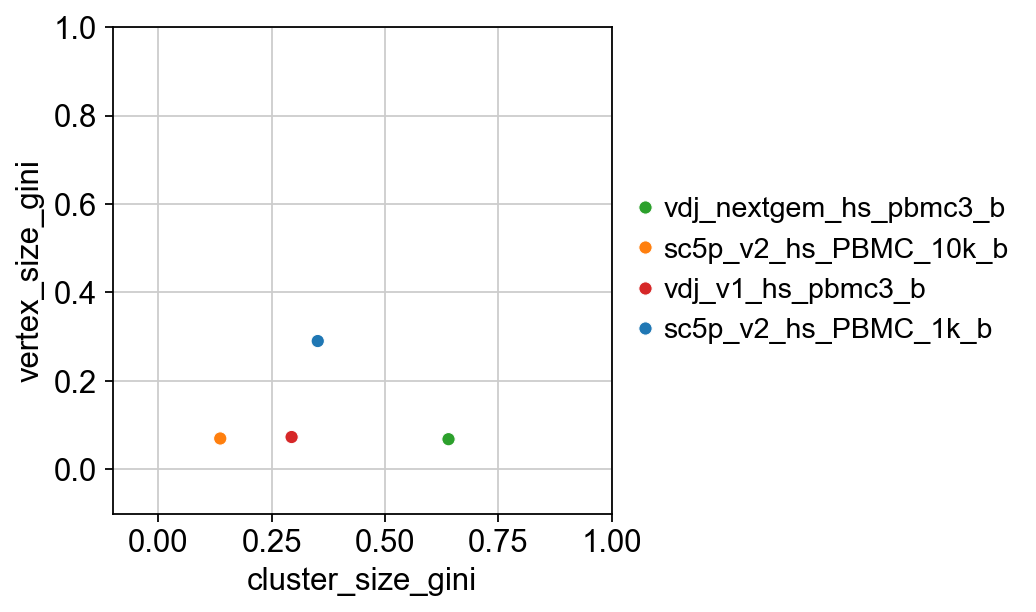
{'cluster_size_gini':                 sample_id      mean       std  lower_95  upper_95
 0  vdj_nextgem_hs_pbmc3_b  0.641934  0.031486  0.578023  0.702337
 1   sc5p_v2_hs_PBMC_10k_b  0.136612  0.018083  0.103946  0.170352
 2       vdj_v1_hs_pbmc3_b  0.298734  0.029397  0.249417  0.352936
 3    sc5p_v2_hs_PBMC_1k_b  0.337680  0.024345  0.290320  0.389317,
 'vertex_size_gini':                 sample_id      mean       std  lower_95  upper_95
 0  vdj_nextgem_hs_pbmc3_b  0.070595  0.017534  0.036411  0.106486
 1   sc5p_v2_hs_PBMC_10k_b  0.070233  0.014536  0.043873  0.096845
 2       vdj_v1_hs_pbmc3_b  0.078035  0.047738  0.035441  0.206748
 3    sc5p_v2_hs_PBMC_1k_b  0.295633  0.018101  0.256802  0.328979}
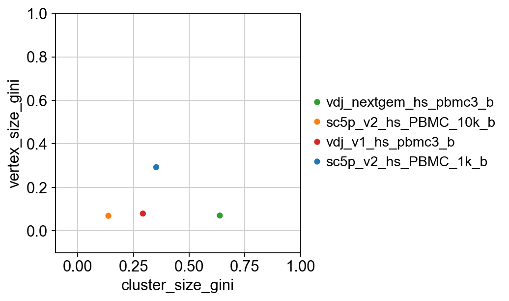
[27]:
# let's merge the two results dataframes for easier plotting
cluster_size = results["cluster_size_gini"][["sample_id", "mean"]]
vertex_size = results["vertex_size_gini"][["sample_id", "mean"]]
cluster_size.rename(columns={"mean": "cluster_size_gini"}, inplace=True)
vertex_size.rename(columns={"mean": "vertex_size_gini"}, inplace=True)
combined_results = pd.concat(
    [cluster_size.set_index("sample_id"), vertex_size.set_index("sample_id")],
    axis=1,
)
# set the colours
palette = dict(
    zip(adata.obs["sample_id"].cat.categories, adata.uns["sample_id_colors"])
)
p = sns.scatterplot(
    x="cluster_size_gini",
    y="vertex_size_gini",
    data=combined_results,
    hue=combined_results.index,
    palette=palette,
)
p.set(ylim=(-0.1, 1), xlim=(-0.1, 1))
plt.legend(bbox_to_anchor=(1, 0.5), loc="center left", frameon=False)
plt.show()
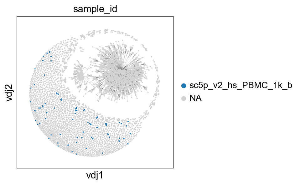
[28]:
ddl.pl.clone_network(
    adata_large, color=["sample_id"], groups=["sc5p_v2_hs_PBMC_1k_b"]
)
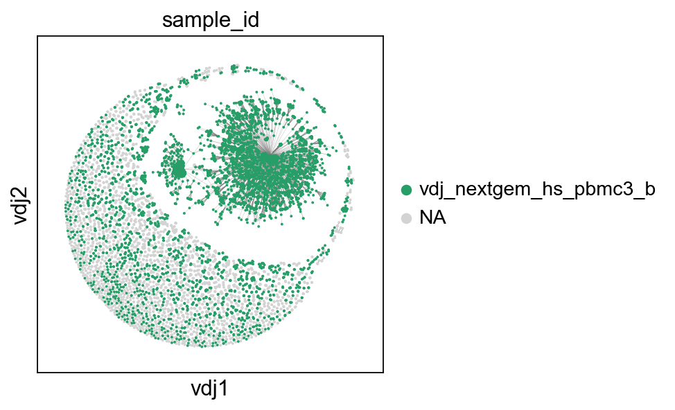
[29]:
ddl.pl.clone_network(
    adata_large, color=["sample_id"], groups=["vdj_nextgem_hs_pbmc3_b"]
)
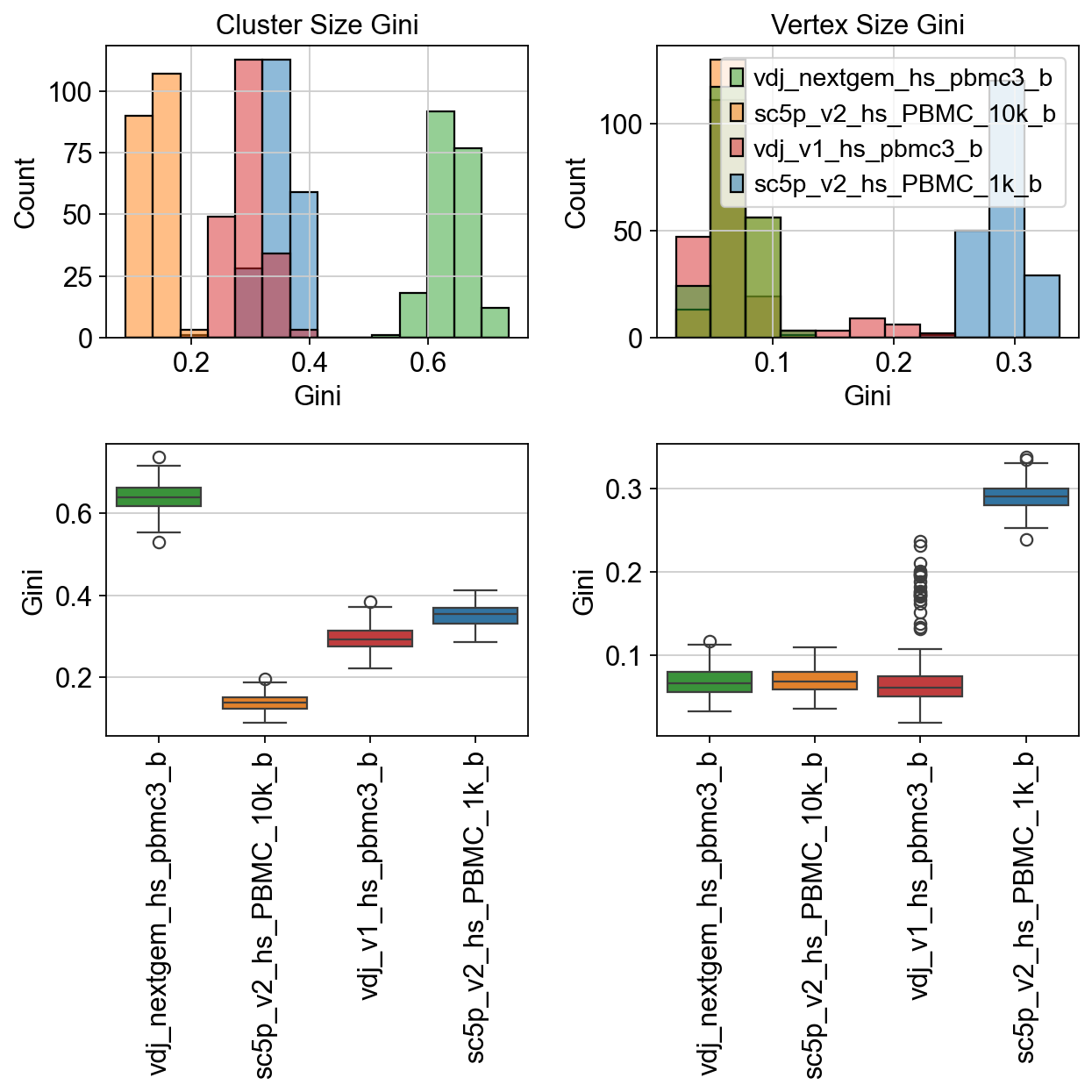
[30]:
fig, axes = plt.subplots(2, 2, figsize=(8, 8))  # 1 row, 2 columns
sns.histplot(
    data=raw["cluster_size_gini"],
    palette=palette,
    ax=axes[0, 0],
)
sns.histplot(
    data=raw["vertex_size_gini"],
    palette=palette,
    ax=axes[0, 1],
)
sns.boxplot(
    data=raw["cluster_size_gini"],
    palette=palette,
    ax=axes[1, 0],
)
sns.boxplot(
    data=raw["vertex_size_gini"],
    palette=palette,
    ax=axes[1, 1],
)
axes[0, 0].set_title("Cluster Size Gini")
axes[0, 1].set_title("Vertex Size Gini")
axes[0, 0].legend_.remove()
axes[0, 0].set_xlabel("Gini")
axes[0, 1].set_xlabel("Gini")
axes[1, 0].set_ylabel("Gini")
axes[1, 1].set_ylabel("Gini")
axes[1, 0].set_xticklabels(axes[1, 0].get_xticklabels(), rotation=90)
axes[1, 1].set_xticklabels(axes[1, 1].get_xticklabels(), rotation=90)
plt.tight_layout()
plt.show()
Now using network_metric = "clone_centrality":
[31]:
results, raw = ddl.tl.clone_diversity(
    vdj_large,
    group_by="sample_id",
    method="gini",
    network_metric="clone_network",
    n_boot=200,
    n_cpus=8,
    verbose=True,
)
results
Calculating Gini indices
Bootstrapping... vdj_nextgem_hs_pbmc3_b: 100%|██████████| 200/200 [00:47<00:00,  4.19it/s]
Bootstrapping... sc5p_v2_hs_PBMC_10k_b: 100%|██████████| 200/200 [00:37<00:00,  5.36it/s]
Bootstrapping... vdj_v1_hs_pbmc3_b: 100%|██████████| 200/200 [00:31<00:00,  6.26it/s]
Bootstrapping... sc5p_v2_hs_PBMC_1k_b: 100%|██████████| 200/200 [00:32<00:00,  6.18it/s]
[31]:
{'cluster_size_gini':                 sample_id      mean       std  lower_95  upper_95
 0  vdj_nextgem_hs_pbmc3_b  0.638076  0.032356  0.575568  0.701389
 1   sc5p_v2_hs_PBMC_10k_b  0.137359  0.018934  0.102266  0.177539
 2       vdj_v1_hs_pbmc3_b  0.300950  0.031542  0.236622  0.357998
 3    sc5p_v2_hs_PBMC_1k_b  0.338231  0.024870  0.284305  0.383072,
 'vertex_size_gini':                 sample_id      mean       std  lower_95  upper_95
 0  vdj_nextgem_hs_pbmc3_b  0.072547  0.017584  0.040410  0.109397
 1   sc5p_v2_hs_PBMC_10k_b  0.070257  0.014201  0.041383  0.096811
 2       vdj_v1_hs_pbmc3_b  0.078298  0.048529  0.035468  0.215533
 3    sc5p_v2_hs_PBMC_1k_b  0.295046  0.018315  0.260065  0.327885}
[32]:
# let's merge the two results dataframes for easier plotting
cluster_size = results["cluster_size_gini"][["sample_id", "mean"]]
vertex_size = results["vertex_size_gini"][["sample_id", "mean"]]
cluster_size.rename(columns={"mean": "cluster_size_gini"}, inplace=True)
vertex_size.rename(columns={"mean": "vertex_size_gini"}, inplace=True)
combined_results = pd.concat(
    [cluster_size.set_index("sample_id"), vertex_size.set_index("sample_id")],
    axis=1,
)
# set the colours
palette = dict(
    zip(adata.obs["sample_id"].cat.categories, adata.uns["sample_id_colors"])
)
p = sns.scatterplot(
    x="cluster_size_gini",
    y="vertex_size_gini",
    data=combined_results,
    hue=combined_results.index,
    palette=palette,
)
p.set(ylim=(-0.1, 1), xlim=(-0.1, 1))
plt.legend(bbox_to_anchor=(1, 0.5), loc="center left", frameon=False)
plt.show()
[33]:
fig, axes = plt.subplots(2, 2, figsize=(8, 8))  # 1 row, 2 columns
sns.histplot(
    data=raw["cluster_size_gini"],
    palette=palette,
    ax=axes[0, 0],
)
sns.histplot(
    data=raw["vertex_size_gini"],
    palette=palette,
    ax=axes[0, 1],
)
sns.boxplot(
    data=raw["cluster_size_gini"],
    palette=palette,
    ax=axes[1, 0],
)
sns.boxplot(
    data=raw["vertex_size_gini"],
    palette=palette,
    ax=axes[1, 1],
)
axes[0, 0].set_title("Cluster Size Gini")
axes[0, 1].set_title("Vertex Size Gini")
axes[0, 0].legend_.remove()
axes[0, 0].set_xlabel("Gini")
axes[0, 1].set_xlabel("Gini")
axes[1, 0].set_ylabel("Gini")
axes[1, 1].set_ylabel("Gini")
axes[1, 0].set_xticklabels(axes[1, 0].get_xticklabels(), rotation=90)
axes[1, 1].set_xticklabels(axes[1, 1].get_xticklabels(), rotation=90)
plt.tight_layout()
plt.show()
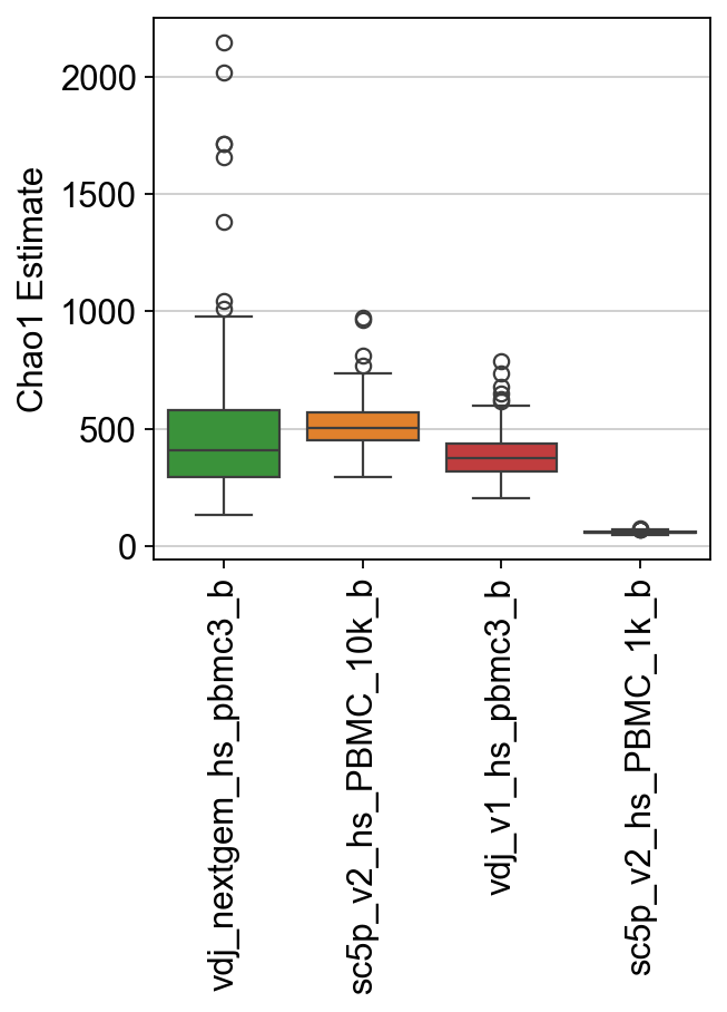
Finally, let’s try the other diversity methods. chao1 is an estimator based on abundance.
[34]:
results, raw = ddl.tl.clone_diversity(
    vdj_large,
    group_by="sample_id",
    method="chao1",
    n_boot=200,
    n_cpus=8,
    verbose=True,
)
results
Bootstrapping… vdj_nextgem_hs_pbmc3_b: 100%|██████████| 200/200 [00:01<00:00, 127.85it/s]
Bootstrapping… sc5p_v2_hs_PBMC_10k_b: 100%|██████████| 200/200 [00:00<00:00, 829.15it/s]
Bootstrapping… vdj_v1_hs_pbmc3_b: 100%|██████████| 200/200 [00:00<00:00, 962.52it/s]
Bootstrapping… sc5p_v2_hs_PBMC_1k_b: 100%|██████████| 200/200 [00:00<00:00, 4579.91it/s]
[34]:
{'chao1':                 sample_id        mean         std    lower_95     upper_95
 0  vdj_nextgem_hs_pbmc3_b  483.501125  275.413592  193.107500  1278.087500
 1   sc5p_v2_hs_PBMC_10k_b  515.477668  104.990081  346.029215   746.024588
 2       vdj_v1_hs_pbmc3_b  370.102085   76.168531  252.867618   545.941786
 3    sc5p_v2_hs_PBMC_1k_b   61.621807    5.354899   53.293576    72.157500}
[35]:
ax = sns.boxplot(
    data=raw["chao1"],
    palette=palette,
)
ax.set_ylabel("Chao1 Estimate")
ax.set_xticklabels(ax.get_xticklabels(), rotation=90)
plt.show()
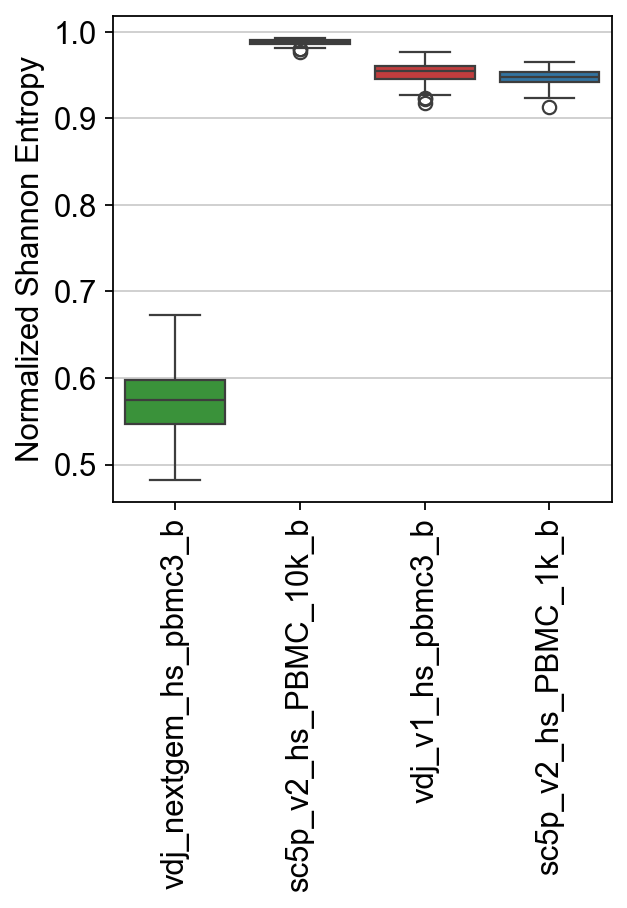
For Shannon Entropy, we can calculate a normalized (inspired by scirpy’s function) and non-normalized value.
[36]:
results, raw = ddl.tl.clone_diversity(
    vdj_large,
    group_by="sample_id",
    method="shannon",
    n_boot=200,
    n_cpus=8,
    verbose=True,
)
results
Bootstrapping… vdj_nextgem_hs_pbmc3_b: 100%|██████████| 200/200 [00:01<00:00, 112.92it/s]
Bootstrapping… sc5p_v2_hs_PBMC_10k_b: 100%|██████████| 200/200 [00:00<00:00, 687.28it/s]
Bootstrapping… vdj_v1_hs_pbmc3_b: 100%|██████████| 200/200 [00:00<00:00, 802.55it/s]
Bootstrapping… sc5p_v2_hs_PBMC_1k_b: 100%|██████████| 200/200 [00:00<00:00, 4010.25it/s]
[36]:
{'shannon':                 sample_id      mean       std  lower_95  upper_95
 0  vdj_nextgem_hs_pbmc3_b  0.568512  0.033453  0.496321  0.625179
 1   sc5p_v2_hs_PBMC_10k_b  0.987975  0.002604  0.981440  0.992089
 2       vdj_v1_hs_pbmc3_b  0.952263  0.011172  0.927926  0.971630
 3    sc5p_v2_hs_PBMC_1k_b  0.952336  0.007496  0.938674  0.965748}
[37]:
ax = sns.boxplot(
    data=raw["shannon"],
    palette=palette,
)
ax.set_ylabel("Normalized Shannon Entropy")
ax.set_xticklabels(ax.get_xticklabels(), rotation=90)
plt.show()
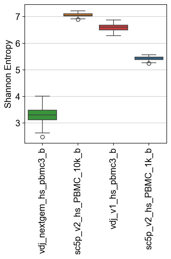
[38]:
results, raw = ddl.tl.clone_diversity(
    vdj_large,
    group_by="sample_id",
    method="shannon",
    n_boot=200,
    n_cpus=8,
    verbose=True,
    normalize=False,
)
results
Bootstrapping… vdj_nextgem_hs_pbmc3_b: 100%|██████████| 200/200 [00:01<00:00, 144.60it/s]
Bootstrapping… sc5p_v2_hs_PBMC_10k_b: 100%|██████████| 200/200 [00:00<00:00, 1016.12it/s]
Bootstrapping… vdj_v1_hs_pbmc3_b: 100%|██████████| 200/200 [00:00<00:00, 1141.14it/s]
Bootstrapping… sc5p_v2_hs_PBMC_1k_b: 100%|██████████| 200/200 [00:00<00:00, 4657.65it/s]
[38]:
{'shannon':                 sample_id      mean       std  lower_95  upper_95
 0  vdj_nextgem_hs_pbmc3_b  3.318948  0.263609  2.835033  3.794615
 1   sc5p_v2_hs_PBMC_10k_b  7.067206  0.056702  6.951599  7.171745
 2       vdj_v1_hs_pbmc3_b  6.587652  0.121024  6.344556  6.801828
 3    sc5p_v2_hs_PBMC_1k_b  5.507010  0.080492  5.323373  5.654755}
[39]:
ax = sns.boxplot(
    data=raw["shannon"],
    palette=palette,
)
ax.set_ylabel("Shannon Entropy")
ax.set_xticklabels(ax.get_xticklabels(), rotation=90)
plt.show()
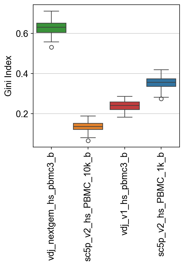
There’s also a gini method that doesn’t require network construction, which should be faster to compute.
[40]:
results, raw = ddl.tl.clone_diversity(
    vdj_large,
    group_by="sample_id",
    method="gini",
    use_network=False,
    n_boot=200,
    n_cpus=8,
    verbose=True,
)
results
Bootstrapping… vdj_nextgem_hs_pbmc3_b: 100%|██████████| 200/200 [00:01<00:00, 130.28it/s]
Bootstrapping… sc5p_v2_hs_PBMC_10k_b: 100%|██████████| 200/200 [00:00<00:00, 860.99it/s]
Bootstrapping… vdj_v1_hs_pbmc3_b: 100%|██████████| 200/200 [00:00<00:00, 1044.61it/s]
Bootstrapping… sc5p_v2_hs_PBMC_1k_b: 100%|██████████| 200/200 [00:00<00:00, 3443.33it/s]
[40]:
{'gini':                 sample_id      mean       std  lower_95  upper_95
 0  vdj_nextgem_hs_pbmc3_b  0.634315  0.031725  0.574024  0.695061
 1   sc5p_v2_hs_PBMC_10k_b  0.134191  0.018743  0.097314  0.166266
 2       vdj_v1_hs_pbmc3_b  0.242385  0.026261  0.190836  0.296391
 3    sc5p_v2_hs_PBMC_1k_b  0.339590  0.026542  0.289624  0.392546}
[41]:
ax = sns.boxplot(
    data=raw["gini"],
    palette=palette,
)
ax.set_ylabel("Gini Index")
ax.set_xticklabels(ax.get_xticklabels(), rotation=90)
plt.show()