V(D)J clustering

On the topic of finding clones/clonotypes, there are many ways used for clustering BCRs, almost all involving some measure based on sequence similarity. There are also a lot of very well established guidelines and criterias maintained by the BCR community. For example, immcantation uses a number of model-based methods [Gupta2015] to group clones based on the distribution of length-normalised junctional hamming distance while others use the whole BCR V(D)J sequence to define clones as shown in this paper [Bashford-Rogers2019].

import os
import scanpy as sc
import dandelion as ddl

ddl.set_backend("base")

os.chdir("dandelion_tutorial")
sc.settings.verbosity = 3

# read in the previously saved file
vdj = ddl.read_h5ddl("dandelion_results.h5ddl")
vdj

Dandelion class object with n_obs = 2493 and n_contigs = 7355
    data: 'sequence_id', 'sequence', 'rev_comp', 'productive', 'v_call', 'd_call', 'j_call', 'sequence_alignment', 'germline_alignment', 'junction', 'junction_aa', 'v_cigar', 'd_cigar', 'j_cigar', 'stop_codon', 'vj_in_frame', 'locus', 'c_call', 'junction_length', 'np1_length', 'np2_length', 'v_sequence_start', 'v_sequence_end', 'v_germline_start', 'v_germline_end', 'd_sequence_start', 'd_sequence_end', 'd_germline_start', 'd_germline_end', 'j_sequence_start', 'j_sequence_end', 'j_germline_start', 'j_germline_end', 'v_score', 'v_identity', 'v_support', 'd_score', 'd_identity', 'd_support', 'j_score', 'j_identity', 'j_support', 'fwr1', 'fwr2', 'fwr3', 'fwr4', 'cdr1', 'cdr2', 'cdr3', 'cell_id', 'consensus_count', 'umi_count', 'v_call_10x', 'd_call_10x', 'j_call_10x', 'junction_10x', 'junction_10x_aa', 'j_support_igblastn', 'j_score_igblastn', 'j_call_igblastn', 'j_call_blastn', 'j_identity_blastn', 'j_alignment_length_blastn', 'j_number_of_mismatches_blastn', 'j_number_of_gap_openings_blastn', 'j_sequence_start_blastn', 'j_sequence_end_blastn', 'j_germline_start_blastn', 'j_germline_end_blastn', 'j_support_blastn', 'j_score_blastn', 'j_sequence_alignment_blastn', 'j_germline_alignment_blastn', 'j_source', 'd_support_igblastn', 'd_score_igblastn', 'd_call_igblastn', 'd_call_blastn', 'd_identity_blastn', 'd_alignment_length_blastn', 'd_number_of_mismatches_blastn', 'd_number_of_gap_openings_blastn', 'd_sequence_start_blastn', 'd_sequence_end_blastn', 'd_germline_start_blastn', 'd_germline_end_blastn', 'd_support_blastn', 'd_score_blastn', 'd_sequence_alignment_blastn', 'd_germline_alignment_blastn', 'd_source', 'v_call_genotyped', 'germline_alignment_d_mask', 'sample_id', 'c_sequence_alignment', 'c_germline_alignment', 'c_sequence_start', 'c_sequence_end', 'c_score', 'c_identity', 'c_call_10x', 'junction_aa_length', 'fwr1_aa', 'fwr2_aa', 'fwr3_aa', 'fwr4_aa', 'cdr1_aa', 'cdr2_aa', 'cdr3_aa', 'sequence_alignment_aa', 'v_sequence_alignment_aa', 'd_sequence_alignment_aa', 'j_sequence_alignment_aa', 'complete_vdj', 'j_call_multimappers', 'j_call_multiplicity', 'j_call_sequence_start_multimappers', 'j_call_sequence_end_multimappers', 'j_call_support_multimappers', 'mu_count', 'ambiguous', 'extra', 'rearrangement_status'
    metadata: 'sample_id', 'locus_VDJ', 'locus_VJ', 'productive_VDJ', 'productive_VJ', 'v_call_VDJ', 'd_call_VDJ', 'j_call_VDJ', 'v_call_VJ', 'j_call_VJ', 'c_call_VDJ', 'c_call_VJ', 'junction_VDJ', 'junction_VJ', 'junction_aa_VDJ', 'junction_aa_VJ', 'v_call_B_VDJ', 'd_call_B_VDJ', 'j_call_B_VDJ', 'v_call_B_VJ', 'j_call_B_VJ', 'c_call_B_VDJ', 'c_call_B_VJ', 'productive_B_VDJ', 'productive_B_VJ', 'umi_count_B_VDJ', 'umi_count_B_VJ', 'v_call_VDJ_main', 'v_call_VJ_main', 'd_call_VDJ_main', 'j_call_VDJ_main', 'j_call_VJ_main', 'c_call_VDJ_main', 'c_call_VJ_main', 'v_call_B_VDJ_main', 'd_call_B_VDJ_main', 'j_call_B_VDJ_main', 'v_call_B_VJ_main', 'j_call_B_VJ_main', 'isotype', 'isotype_status', 'locus_status', 'chain_status', 'rearrangement_status_VDJ', 'rearrangement_status_VJ'

adata = sc.read_h5ad("adata.h5ad")
adata

AnnData object with n_obs × n_vars = 25057 × 1308
    obs: 'sample_id', 'n_genes', 'n_genes_by_counts', 'total_counts', 'total_counts_mt', 'pct_counts_mt', 'gmm_pct_count_clusters_keep', 'scrublet_score', 'is_doublet', 'filter_rna', 'has_contig', 'locus_VDJ', 'locus_VJ', 'productive_VDJ', 'productive_VJ', 'v_call_VDJ', 'd_call_VDJ', 'j_call_VDJ', 'v_call_VJ', 'j_call_VJ', 'c_call_VDJ', 'c_call_VJ', 'junction_VDJ', 'junction_VJ', 'junction_aa_VDJ', 'junction_aa_VJ', 'v_call_B_VDJ', 'd_call_B_VDJ', 'j_call_B_VDJ', 'v_call_B_VJ', 'j_call_B_VJ', 'c_call_B_VDJ', 'c_call_B_VJ', 'productive_B_VDJ', 'productive_B_VJ', 'umi_count_B_VDJ', 'umi_count_B_VJ', 'v_call_VDJ_main', 'v_call_VJ_main', 'd_call_VDJ_main', 'j_call_VDJ_main', 'j_call_VJ_main', 'c_call_VDJ_main', 'c_call_VJ_main', 'v_call_B_VDJ_main', 'd_call_B_VDJ_main', 'j_call_B_VDJ_main', 'v_call_B_VJ_main', 'j_call_B_VJ_main', 'isotype', 'isotype_status', 'locus_status', 'chain_status', 'rearrangement_status_VDJ', 'rearrangement_status_VJ', 'leiden'
    var: 'n_cells', 'highly_variable', 'means', 'dispersions', 'dispersions_norm', 'mean', 'std'
    uns: 'chain_status_colors', 'hvg', 'leiden', 'leiden_colors', 'log1p', 'neighbors', 'pca', 'sample_id_colors', 'umap'
    obsm: 'X_pca', 'X_umap'
    varm: 'PCs'
    obsp: 'connectivities', 'distances'

Finding clones

The following is dandelion’s implementation of a rather conventional method to define clones, ddl.tl.find_clones.

Clone definition criterion

Clone definition is based on the following criterion:

1. Identical V- and J-gene usage in the VDJ chain (IGH/TRB/TRD).

2. Identical CDR3 junctional/CDR3 sequence length in the VDJ chain.

3. VDJ chain junctional/CDR3 sequences attains a minimum of % sequence similarity, based on hamming distance. The similarity cut-off is tunable (default is 85%; change to 100% if analyzing TCR data).

4. VJ chain (IGK/IGL/TRA/TRG) usage. If cells within clones use different VJ chains, the clone will be split following the same conditions for VDJ chains in (1-3) as above.

(Optional) Simplifying annotation calls.

This is an optional step to simplify the annotation calls. The vdj.simplify() will reduce the complexity of the gene names and strip the alleles. This impacts on how clones are defined (using simpler v/j calls) and also visualiation.

# original
vdj.data[["v_call_genotyped", "j_call", "c_call"]]

	v_call_genotyped	j_call	c_call
sequence_id
sc5p_v2_hs_PBMC_10k_b_AAACCTGTCATATCGG_contig_1	IGKV1-33*01,IGKV1D-33*01	IGKJ4*01	IGKC
sc5p_v2_hs_PBMC_10k_b_AAACCTGTCCGTTGTC_contig_2	IGHV1-69*01,IGHV1-69D*01	IGHJ3*02	IGHM
sc5p_v2_hs_PBMC_10k_b_AAACCTGTCCGTTGTC_contig_1	IGKV1-8*01	IGKJ1*01	IGKC
sc5p_v2_hs_PBMC_10k_b_AAACCTGTCGAGAACG_contig_1	IGLV5-45*02	IGLJ3*02	IGLC3
sc5p_v2_hs_PBMC_10k_b_AAACCTGTCGAGAACG_contig_2	IGHV1-2*02	IGHJ3*02	IGHM
...	...	...	...
vdj_v1_hs_pbmc3_b_TTTCCTCTCGACAGCC_contig_1	IGHV1-46*01	IGHJ5*02	IGHM
vdj_v1_hs_pbmc3_b_TTTGCGCCATACCATG_contig_2	IGHV1-69*01,IGHV1-69D*01	IGHJ6*02	IGHM
vdj_v1_hs_pbmc3_b_TTTGCGCCATACCATG_contig_1	IGLV1-47*01	IGLJ3*02	IGLC3
vdj_v1_hs_pbmc3_b_TTTGGTTGTAGGCATG_contig_2	IGLV2-11*01	IGLJ2*01,IGLJ3*01,IGLJ3*02	IGLC
vdj_v1_hs_pbmc3_b_TTTGGTTGTAGGCATG_contig_1	IGHV3-23*01,IGHV3-23D*01	IGHJ4*02	IGHM

7355 rows × 3 columns

vdj.simplify()
vdj.data[["v_call_genotyped", "j_call", "c_call"]]

	v_call_genotyped	j_call	c_call
sequence_id
sc5p_v2_hs_PBMC_10k_b_AAACCTGTCATATCGG_contig_1	IGKV1-33	IGKJ4	IGKC
sc5p_v2_hs_PBMC_10k_b_AAACCTGTCCGTTGTC_contig_2	IGHV1-69	IGHJ3	IGHM
sc5p_v2_hs_PBMC_10k_b_AAACCTGTCCGTTGTC_contig_1	IGKV1-8	IGKJ1	IGKC
sc5p_v2_hs_PBMC_10k_b_AAACCTGTCGAGAACG_contig_1	IGLV5-45	IGLJ3	IGLC3
sc5p_v2_hs_PBMC_10k_b_AAACCTGTCGAGAACG_contig_2	IGHV1-2	IGHJ3	IGHM
...	...	...	...
vdj_v1_hs_pbmc3_b_TTTCCTCTCGACAGCC_contig_1	IGHV1-46	IGHJ5	IGHM
vdj_v1_hs_pbmc3_b_TTTGCGCCATACCATG_contig_2	IGHV1-69	IGHJ6	IGHM
vdj_v1_hs_pbmc3_b_TTTGCGCCATACCATG_contig_1	IGLV1-47	IGLJ3	IGLC3
vdj_v1_hs_pbmc3_b_TTTGGTTGTAGGCATG_contig_2	IGLV2-11	IGLJ2	IGLC
vdj_v1_hs_pbmc3_b_TTTGGTTGTAGGCATG_contig_1	IGHV3-23	IGHJ4	IGHM

7355 rows × 3 columns

# let's save this as a separate file
vdj.write_h5ddl("dandelion_results_simplified.h5ddl", compression="gzip")

Running ddl.tl.find_clones

The function will take a file path, a pandas DataFrame (for example if you’ve used pandas to read in the filtered file already), or a Dandelion class object. The default mode for calculation of junctional hamming distance is to use the CDR3 junction amino acid sequences, specified via the key option (None defaults to junction_aa). You can switch it to using CDR3 junction nucleotide sequences (key = 'junction'), or even the full V(D)J amino acid sequence (key = 'sequence_alignment_aa'), as long as the column name exists in the .data slot.

Clustering TCR is possible with the same setup but requires changing of default parameters (covered in the TCR section).

ddl.tl.find_clones(vdj)
vdj

Finding clonotypes

Finding clones based on B cell VDJ chains using junction_aa: 100%|██████████| 200/200 [00:00<00:00, 1678.84it/s]
Finding clones based on B cell VJ chains using junction_aa: 100%|██████████| 207/207 [00:00<00:00, 3385.96it/s]
Refining clone assignment based on VJ chain pairing : 100%|██████████| 2493/2493 [00:00<00:00, 374164.46it/s]

Initialising Dandelion object
 finished: Updated Dandelion object:
   'data', contig-indexed AIRR table
   'metadata', cell-indexed observations table
 (0:00:02)

Dandelion class object with n_obs = 2493 and n_contigs = 7355
    data: 'sequence_id', 'sequence', 'rev_comp', 'productive', 'v_call', 'd_call', 'j_call', 'sequence_alignment', 'germline_alignment', 'junction', 'junction_aa', 'v_cigar', 'd_cigar', 'j_cigar', 'stop_codon', 'vj_in_frame', 'locus', 'c_call', 'junction_length', 'np1_length', 'np2_length', 'v_sequence_start', 'v_sequence_end', 'v_germline_start', 'v_germline_end', 'd_sequence_start', 'd_sequence_end', 'd_germline_start', 'd_germline_end', 'j_sequence_start', 'j_sequence_end', 'j_germline_start', 'j_germline_end', 'v_score', 'v_identity', 'v_support', 'd_score', 'd_identity', 'd_support', 'j_score', 'j_identity', 'j_support', 'fwr1', 'fwr2', 'fwr3', 'fwr4', 'cdr1', 'cdr2', 'cdr3', 'cell_id', 'consensus_count', 'umi_count', 'v_call_10x', 'd_call_10x', 'j_call_10x', 'junction_10x', 'junction_10x_aa', 'j_support_igblastn', 'j_score_igblastn', 'j_call_igblastn', 'j_call_blastn', 'j_identity_blastn', 'j_alignment_length_blastn', 'j_number_of_mismatches_blastn', 'j_number_of_gap_openings_blastn', 'j_sequence_start_blastn', 'j_sequence_end_blastn', 'j_germline_start_blastn', 'j_germline_end_blastn', 'j_support_blastn', 'j_score_blastn', 'j_sequence_alignment_blastn', 'j_germline_alignment_blastn', 'j_source', 'd_support_igblastn', 'd_score_igblastn', 'd_call_igblastn', 'd_call_blastn', 'd_identity_blastn', 'd_alignment_length_blastn', 'd_number_of_mismatches_blastn', 'd_number_of_gap_openings_blastn', 'd_sequence_start_blastn', 'd_sequence_end_blastn', 'd_germline_start_blastn', 'd_germline_end_blastn', 'd_support_blastn', 'd_score_blastn', 'd_sequence_alignment_blastn', 'd_germline_alignment_blastn', 'd_source', 'v_call_genotyped', 'germline_alignment_d_mask', 'sample_id', 'c_sequence_alignment', 'c_germline_alignment', 'c_sequence_start', 'c_sequence_end', 'c_score', 'c_identity', 'c_call_10x', 'junction_aa_length', 'fwr1_aa', 'fwr2_aa', 'fwr3_aa', 'fwr4_aa', 'cdr1_aa', 'cdr2_aa', 'cdr3_aa', 'sequence_alignment_aa', 'v_sequence_alignment_aa', 'd_sequence_alignment_aa', 'j_sequence_alignment_aa', 'complete_vdj', 'j_call_multimappers', 'j_call_multiplicity', 'j_call_sequence_start_multimappers', 'j_call_sequence_end_multimappers', 'j_call_support_multimappers', 'mu_count', 'ambiguous', 'extra', 'rearrangement_status', 'clone_id'
    metadata: 'clone_id', 'clone_id_rank', 'sample_id', 'locus_VDJ', 'locus_VJ', 'productive_VDJ', 'productive_VJ', 'v_call_VDJ', 'd_call_VDJ', 'j_call_VDJ', 'v_call_VJ', 'j_call_VJ', 'c_call_VDJ', 'c_call_VJ', 'junction_VDJ', 'junction_VJ', 'junction_aa_VDJ', 'junction_aa_VJ', 'v_call_B_VDJ', 'd_call_B_VDJ', 'j_call_B_VDJ', 'v_call_B_VJ', 'j_call_B_VJ', 'c_call_B_VDJ', 'c_call_B_VJ', 'productive_B_VDJ', 'productive_B_VJ', 'umi_count_B_VDJ', 'umi_count_B_VJ', 'v_call_VDJ_main', 'v_call_VJ_main', 'd_call_VDJ_main', 'j_call_VDJ_main', 'j_call_VJ_main', 'c_call_VDJ_main', 'c_call_VJ_main', 'v_call_B_VDJ_main', 'd_call_B_VDJ_main', 'j_call_B_VDJ_main', 'v_call_B_VJ_main', 'j_call_B_VJ_main', 'isotype', 'isotype_status', 'locus_status', 'chain_status', 'rearrangement_status_VDJ', 'rearrangement_status_VJ'

This will return a new column with the column name 'clone_id' as per convention. If a file path is provided as input, it will also save the file automatically into the base directory of the file name. Otherwise, a Dandelion object will be returned.

Clonotype definition criterion

The clone_id follows an VDJ_{A}_{B}_{C}_VJ_{D}_{E}_{F} format and largely reflects the conditions above where:

{A} indicates if the contigs use the same V and J genes in the VDJ chain.

{B} indicates if junctional/CDR3 sequences are equal in length in the VDJ chain.

{C} indicates if clones are split based on junctional/CDR3 hamming distance threshold (for VDJ chain).

{D} indicates if the contigs use the same V and J genes in the VJ chain.

{E} indicates if junctional/CDR3 sequences are equal in length in the VJ chain.

{F} indicates if clones are split based on junctional/CDR3 hamming distance threshold (for VJ chain).

Also, to prevent issues with clonotype ids matching between B cells and T cells, there will be a prefix added to the clone_id to reflect whether or not it’s a B, abT or gdT clone.

Therefor, a complete B cell clonotype id will look something like:

B_VDJ_1_1_2_VJ_2_1_1

For an Orphan VDJ, it would be B_VDJ_1_1_2.

For an Orphan VJ, it would be B_VJ_2_1_1.

The individual numbers in the clonotype id do not have any meaning on their own, other than to indicate whether or not the conditions were met. For example, a 1 in the first position indicates that all contigs in that clone use the same V and J genes in the VDJ chain, while a 2 indicates that there that clone uses a different set of V/J genes.

There are different defaults depending on the type of receptor data being analysed. For BCR data, the default identity threshold is set to 0.85 (i.e. 85% similarity based on hamming distance) while for TCR data, the default is set to 1.0 (i.e. 100% similarity). BCR uses junction_aa (amino acid) as the default key for calculating hamming distance while TCR uses junction (nucleotide) as default. These two parameters can be changed via the identity and key options respectively, which accepts a dictionary for each receptor type like so:

ddl.tl.find_clones(vdj,
    identity = {'ig': 0.85, 'tr-ab': 1.0, 'tr-gd': 1.0},
    key = {'ig': 'junction_aa', 'tr-ab': 'junction', 'tr-gd': 'junction'}
)

This also means that ddl.tl.find_clones can be used for data containing both BCR and TCR data in the same object and the appropriate parameters will be applied to each receptor type accordingly.

There is also an alternate column called clone_id_rank which is a simplified numerical version of the clone_id which corresponds to the size of the clonotype - 1 is the largest clonotype, 2 is the second largest, and so on. Numbering is done separately for each receptor type if there are multiple receptor types in the data, i.e. it would look like B_1, B_2, abT_1, etc. There is a separate tutorial on handling multi-receptor data at here that will go into more details.

vdj.metadata

	clone_id	clone_id_rank	sample_id	locus_VDJ	locus_VJ	productive_VDJ	productive_VJ	v_call_VDJ	d_call_VDJ	j_call_VDJ	...	d_call_B_VDJ_main	j_call_B_VDJ_main	v_call_B_VJ_main	j_call_B_VJ_main	isotype	isotype_status	locus_status	chain_status	rearrangement_status_VDJ	rearrangement_status_VJ
sc5p_v2_hs_PBMC_10k_b_AAACCTGTCATATCGG	B_VJ_127_2_2	135	sc5p_v2_hs_PBMC_10k_b	None	IGK	None	T	None	None	None	...	None	None	IGKV1-33	IGKJ4	None	None	Orphan IGK	Orphan VJ	None	standard
sc5p_v2_hs_PBMC_10k_b_AAACCTGTCCGTTGTC	B_VDJ_151_4_1_VJ_151_2_1	2196	sc5p_v2_hs_PBMC_10k_b	IGH	IGK	T	T	IGHV1-69	IGHD3-22	IGHJ3	...	IGHD3-22	IGHJ3	IGKV1-8	IGKJ1	IgM	IgM	IGH + IGK	Single pair	standard	standard
sc5p_v2_hs_PBMC_10k_b_AAACCTGTCGAGAACG	B_VDJ_1_1_1_VJ_33_1_1	1750	sc5p_v2_hs_PBMC_10k_b	IGH	IGL	T	T	IGHV1-2	None	IGHJ3	...	None	IGHJ3	IGLV5-45	IGLJ3	IgM	IgM	IGH + IGL	Single pair	standard	standard
sc5p_v2_hs_PBMC_10k_b_AAACCTGTCTTGAGAC	B_VDJ_152_4_2_VJ_84_1_1	1751	sc5p_v2_hs_PBMC_10k_b	IGH	IGK	T	T	IGHV5-51	None	IGHJ3	...	None	IGHJ3	IGKV1D-8	IGKJ2	IgM	IgM	IGH + IGK	Single pair	standard	standard
sc5p_v2_hs_PBMC_10k_b_AAACGGGAGCGACGTA	B_VDJ_31_2_1_VJ_4_2_1	1752	sc5p_v2_hs_PBMC_10k_b	IGH	IGL	T	T	IGHV4-4	IGHD6-13	IGHJ3	...	IGHD6-13	IGHJ3	IGLV3-19	IGLJ2	IgM	IgM	IGH + IGL	Single pair	standard	standard
...	...	...	...	...	...	...	...	...	...	...	...	...	...	...	...	...	...	...	...	...	...
vdj_v1_hs_pbmc3_b_TTTCCTCAGCGCTTAT	B_VDJ_173_5_6_VJ_47_1_1	895	vdj_v1_hs_pbmc3_b	IGH	IGK	T	T	IGHV3-30	IGHD4-17	IGHJ6	...	IGHD4-17	IGHJ6	IGKV2-30	IGKJ2	IgM	IgM	IGH + IGK	Single pair	standard	standard
vdj_v1_hs_pbmc3_b_TTTCCTCAGGGAAACA	B_VDJ_6_2_1_VJ_109_4_1	896	vdj_v1_hs_pbmc3_b	IGH	IGK	T	T	IGHV4-61	IGHD6-13	IGHJ2	...	IGHD6-13	IGHJ2	IGKV1-39	IGKJ1	IgM	IgM	IGH + IGK	Single pair	standard	standard
vdj_v1_hs_pbmc3_b_TTTCCTCTCGACAGCC	B_VDJ_16_5_1_VJ_95_2_1	897	vdj_v1_hs_pbmc3_b	IGH	IGK	T	T	IGHV1-46	IGHD2-15	IGHJ5	...	IGHD2-15	IGHJ5	IGKV1-39	IGKJ2	IgM	IgM	IGH + IGK	Single pair	standard	standard
vdj_v1_hs_pbmc3_b_TTTGCGCCATACCATG	B_VDJ_183_7_2_VJ_149_3_1	898	vdj_v1_hs_pbmc3_b	IGH	IGL	T	T	IGHV1-69	IGHD2-15	IGHJ6	...	IGHD2-15	IGHJ6	IGLV1-47	IGLJ3	IgM	IgM	IGH + IGL	Single pair	standard	standard
vdj_v1_hs_pbmc3_b_TTTGGTTGTAGGCATG	B_VDJ_35_6_7_VJ_45_3_1	2598	vdj_v1_hs_pbmc3_b	IGH	IGL	T	T	IGHV3-23	None	IGHJ4	...	None	IGHJ4	IGLV2-11	IGLJ2	IgM	IgM	IGH + IGL	Single pair	standard	standard

2493 rows × 47 columns

Alternative : Running ddl.tl.define_clones

Alternatively, a wrapper to call changeo’s DefineClones.py [Gupta2015] is also included. To run it, you need to choose the distance threshold for clonal assignment. To facilitate this, the function ddl.pp.calculate_threshold will run shazam’s distToNearest function and return a plot showing the length normalized hamming distance distribution and automated threshold value.

For more fine control, please use shazam’s distToNearest and changeo’s DefineClones.py functions directly.

threshold = ddl.pp.calculate_threshold(vdj)
print(f"clone distance threshold: {threshold}")

Calculating threshold

R[write to console]: Error in (function (db, sequenceColumn = "junction", vCallColumn = "v_call",  :
  361 cell(s) with multiple heavy chains found. One heavy chain per cell is expected.

Rerun this after filtering. For now, switching to heavy mode.

R[write to console]: Running in non-single-cell mode.

      Threshold method 'density' did not return with any values. Switching to method = 'gmm'.

/opt/homebrew/Caskroom/miniforge/base/envs/dandelion/lib/python3.12/site-packages/plotnine/layer.py:284: PlotnineWarning: stat_bin : Removed 921 rows containing non-finite values.

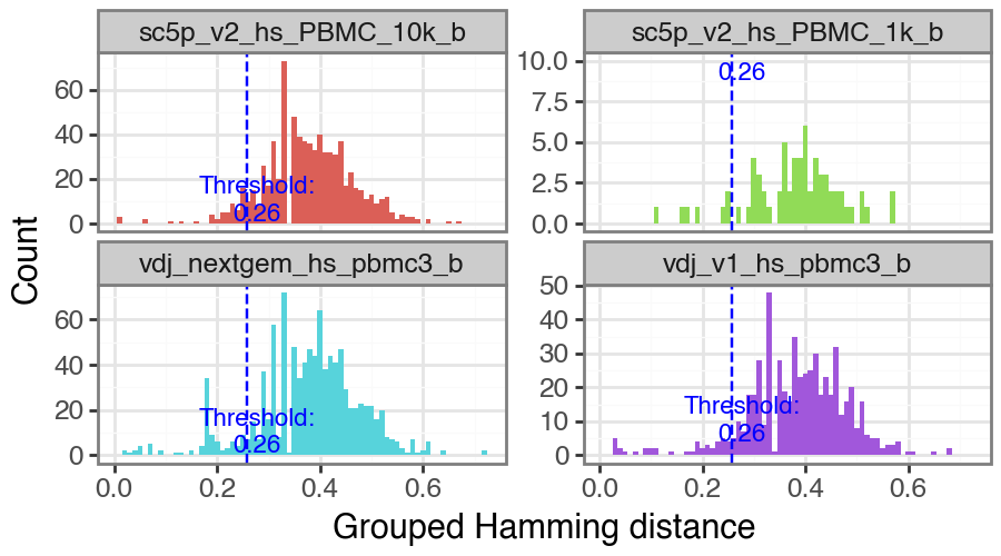
clone distance threshold: 0.2570795622859657

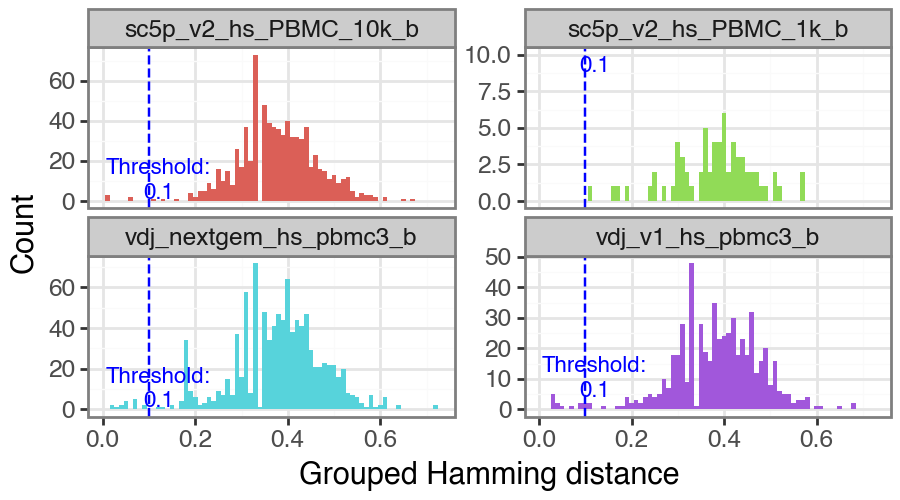
You can also manually select a value as the threshold if you wish. Note that rerunning this with manual_threshold is just for reproducing the plot but with the line at 0.1 in this tutorial.

_ = ddl.pp.calculate_threshold(vdj, manual_threshold=0.1)

Calculating threshold

R[write to console]: Error in (function (db, sequenceColumn = "junction", vCallColumn = "v_call",  :
  361 cell(s) with multiple heavy chains found. One heavy chain per cell is expected.

Rerun this after filtering. For now, switching to heavy mode.

R[write to console]: Running in non-single-cell mode.

/opt/homebrew/Caskroom/miniforge/base/envs/dandelion/lib/python3.12/site-packages/plotnine/layer.py:284: PlotnineWarning: stat_bin : Removed 921 rows containing non-finite values.

We can run ddl.tl.define_clones to call changeo’s DefineClones.py; see here for more info. The value in dist option (corresponds to threshold value) needs to be manually supplied. Additional options for ddl.tl.define_clones to provide to DefineClones.py can be supplied as a list to the additional_args option.

# make a copy of the original vdj object to compare results
vdj_changeo = vdj.copy()
ddl.tl.define_clones(vdj_changeo, dist=threshold, key_added="changeo_clone_id")
vdj_changeo

Finding clones
Running command: DefineClones.py -d /var/folders/_r/j_8_fj3x28n2th3ch0ckn9c40000gt/T/tmpkx18kkga/tmp/dandelion_define_clones_heavy-clone.tsv -o /var/folders/_r/j_8_fj3x28n2th3ch0ckn9c40000gt/T/tmpkx18kkga/dandelion_define_clones_heavy-clone.tsv --act set --model ham --norm len --dist 0.2570795622859657 --nproc 1 --vf v_call_genotyped

       START> DefineClones
        FILE> dandelion_define_clones_heavy-clone.tsv
   SEQ_FIELD> junction
     V_FIELD> v_call_genotyped
     J_FIELD> j_call
 MAX_MISSING> 0
GROUP_FIELDS> None
      ACTION> set
        MODE> gene
    DISTANCE> 0.2570795622859657
     LINKAGE> single
       MODEL> ham
        NORM> len
         SYM> avg
       NPROC> 1

PROGRESS> [Grouping sequences] 15:52:57 (2402) 0.0 min

PROGRESS> [Assigning clones] 15:52:59 |####################| 100% (2,402) 0.0 min

 OUTPUT> dandelion_define_clones_heavy-clone.tsv
 CLONES> 2260
RECORDS> 2402
   PASS> 2402
   FAIL> 0
    END> DefineClones

 finished: Updated Dandelion object:
   'data', contig-indexed AIRR table
   'metadata', cell-indexed observations table
 (0:00:10)

Dandelion class object with n_obs = 2493 and n_contigs = 7355
    data: 'sequence_id', 'sequence', 'rev_comp', 'productive', 'v_call', 'd_call', 'j_call', 'sequence_alignment', 'germline_alignment', 'junction', 'junction_aa', 'v_cigar', 'd_cigar', 'j_cigar', 'stop_codon', 'vj_in_frame', 'locus', 'c_call', 'junction_length', 'np1_length', 'np2_length', 'v_sequence_start', 'v_sequence_end', 'v_germline_start', 'v_germline_end', 'd_sequence_start', 'd_sequence_end', 'd_germline_start', 'd_germline_end', 'j_sequence_start', 'j_sequence_end', 'j_germline_start', 'j_germline_end', 'v_score', 'v_identity', 'v_support', 'd_score', 'd_identity', 'd_support', 'j_score', 'j_identity', 'j_support', 'fwr1', 'fwr2', 'fwr3', 'fwr4', 'cdr1', 'cdr2', 'cdr3', 'cell_id', 'consensus_count', 'umi_count', 'v_call_10x', 'd_call_10x', 'j_call_10x', 'junction_10x', 'junction_10x_aa', 'j_support_igblastn', 'j_score_igblastn', 'j_call_igblastn', 'j_call_blastn', 'j_identity_blastn', 'j_alignment_length_blastn', 'j_number_of_mismatches_blastn', 'j_number_of_gap_openings_blastn', 'j_sequence_start_blastn', 'j_sequence_end_blastn', 'j_germline_start_blastn', 'j_germline_end_blastn', 'j_support_blastn', 'j_score_blastn', 'j_sequence_alignment_blastn', 'j_germline_alignment_blastn', 'j_source', 'd_support_igblastn', 'd_score_igblastn', 'd_call_igblastn', 'd_call_blastn', 'd_identity_blastn', 'd_alignment_length_blastn', 'd_number_of_mismatches_blastn', 'd_number_of_gap_openings_blastn', 'd_sequence_start_blastn', 'd_sequence_end_blastn', 'd_germline_start_blastn', 'd_germline_end_blastn', 'd_support_blastn', 'd_score_blastn', 'd_sequence_alignment_blastn', 'd_germline_alignment_blastn', 'd_source', 'v_call_genotyped', 'germline_alignment_d_mask', 'sample_id', 'c_sequence_alignment', 'c_germline_alignment', 'c_sequence_start', 'c_sequence_end', 'c_score', 'c_identity', 'c_call_10x', 'junction_aa_length', 'fwr1_aa', 'fwr2_aa', 'fwr3_aa', 'fwr4_aa', 'cdr1_aa', 'cdr2_aa', 'cdr3_aa', 'sequence_alignment_aa', 'v_sequence_alignment_aa', 'd_sequence_alignment_aa', 'j_sequence_alignment_aa', 'complete_vdj', 'j_call_multimappers', 'j_call_multiplicity', 'j_call_sequence_start_multimappers', 'j_call_sequence_end_multimappers', 'j_call_support_multimappers', 'mu_count', 'ambiguous', 'extra', 'rearrangement_status', 'clone_id', 'changeo_clone_id'
    metadata: 'changeo_clone_id', 'changeo_clone_id_rank', 'clone_id', 'clone_id_rank', 'sample_id', 'locus_VDJ', 'locus_VJ', 'productive_VDJ', 'productive_VJ', 'v_call_VDJ', 'd_call_VDJ', 'j_call_VDJ', 'v_call_VJ', 'j_call_VJ', 'c_call_VDJ', 'c_call_VJ', 'junction_VDJ', 'junction_VJ', 'junction_aa_VDJ', 'junction_aa_VJ', 'v_call_B_VDJ', 'd_call_B_VDJ', 'j_call_B_VDJ', 'v_call_B_VJ', 'j_call_B_VJ', 'c_call_B_VDJ', 'c_call_B_VJ', 'productive_B_VDJ', 'productive_B_VJ', 'umi_count_B_VDJ', 'umi_count_B_VJ', 'v_call_VDJ_main', 'v_call_VJ_main', 'd_call_VDJ_main', 'j_call_VDJ_main', 'j_call_VJ_main', 'c_call_VDJ_main', 'c_call_VJ_main', 'v_call_B_VDJ_main', 'd_call_B_VDJ_main', 'j_call_B_VDJ_main', 'v_call_B_VJ_main', 'j_call_B_VJ_main', 'isotype', 'isotype_status', 'locus_status', 'chain_status', 'rearrangement_status_VDJ', 'rearrangement_status_VJ'

Note that I specified the parameter key_added and this adds the clone id output from ddl.tl.define_clones into a separate column. If left as default (None), it will write into clone_id column. The same key_added parameter can be specified in ddl.tl.find_clones earlier. You will notice that vdj_changeo is initisalised with changeo_clone_id as the first column while vdj has clone_id as the first.

Other clustering methods

dandelion also now supports clustering methods from scoper. You can access the functions through:

dandelion.external.immcancation.scoper.identical_clones(vdj, ...)
dandelion.external.immcancation.scoper.hierarchical_clones(vdj, ...)
dandelion.external.immcancation.scoper.spectral_clones(vdj, ...)

see the dandelion documentation and original scoper documentation for more details.

As more methods arise, we will continue to evaluate which ones to include in dandelion.

Generation of V(D)J network

dandelion generates a network to facilitate visualisation of results, inspired from [Bashford-Rogers2013]. The deafult uses the full V(D)J contig amino acid sequences to chart a tree-like network for each clone, but it can also be used on any sequence columns, e.g. junctional nucleotide sequences. The actual visualization will be achieved through scanpy later.

ddl.tl.generate_network

First we need to generate the network. ddl.tl.generate_network will take a V(D)J table that has clones defined, specifically under the clone_id column. The default mode is to use amino acid sequences for constructing Levenshtein distance matrices, but can be toggled using the key option, as well as other options for distance calculation, which will be covered in a separate tutorial later.

If you have a pre-processed table parsed from immcantation’s method, or any other method as long as it’s in AIRR format, the table can be used as well.

You can specify the clone_key option for generating the network for the clone id definition of choice as long as it exists as a column in the .data slot.

In version 1.0.0 onwards, the method for distance calculation has been refactored to improve the speed. Prior to this, the distance matrix was always computed on a per chain basis and done sequentially as a loop over each chain. We have now vectorized the distance calculation to compute the distances for all chains at once while accounting for gaps, which should significantly speed up the process. There’s also an option to use n_cpus to parallelize the computation across multiple cores, as well as the ability to supply a lambda function for custom distance calculation, or calculating BLOSUM-based distances. We will cover these options in more details in a later tutorial.

Layout Method Updates

Several new layout algorithm options are available:

Method	Description
mod_fr	Original Python modified Fruchterman-Reingold layout
mod_fr2	New default. Numba-accelerated FR layout (faster on CPU)
mod_fr2_gpu	PyTorch GPU-accelerated FR (auto-tiles for >100K nodes)
mod_fr_bh	Barnes-Hut O(N log N) CPU layout (scalable for large graphs)
mod_fr_bh_gpu	Barnes-Hut GPU layout (requires CUDA)
fa2	ForceAtlas2 (requires fa2-modified)

The singleton_mass parameter (default 0.5) controls the mass of isolated nodes in Barnes-Hut layouts. Lowering this reduces the repulsive force that singletons exert on connected components.

Before proceeding, let’s do a bit of subsetting. Here I want to remove the Orphan VJ cells (lacking BCR heavy chain i.e. VDJ information). Whether or not you want to do this is up to you. I’m doing this because I want to focus on the BCR heavy chain for now. You may elect to keep everything and that can be your starting point for further analysis.

vdj = vdj[
    vdj.metadata.chain_status.isin(
        ["Single pair", "Extra pair", "Extra pair-exception", "Orphan VDJ"]
    )
].copy()
vdj

Dandelion class object with n_obs = 2334 and n_contigs = 5557
    data: 'sequence_id', 'sequence', 'rev_comp', 'productive', 'v_call', 'd_call', 'j_call', 'sequence_alignment', 'germline_alignment', 'junction', 'junction_aa', 'v_cigar', 'd_cigar', 'j_cigar', 'stop_codon', 'vj_in_frame', 'locus', 'c_call', 'junction_length', 'np1_length', 'np2_length', 'v_sequence_start', 'v_sequence_end', 'v_germline_start', 'v_germline_end', 'd_sequence_start', 'd_sequence_end', 'd_germline_start', 'd_germline_end', 'j_sequence_start', 'j_sequence_end', 'j_germline_start', 'j_germline_end', 'v_score', 'v_identity', 'v_support', 'd_score', 'd_identity', 'd_support', 'j_score', 'j_identity', 'j_support', 'fwr1', 'fwr2', 'fwr3', 'fwr4', 'cdr1', 'cdr2', 'cdr3', 'cell_id', 'consensus_count', 'umi_count', 'v_call_10x', 'd_call_10x', 'j_call_10x', 'junction_10x', 'junction_10x_aa', 'j_support_igblastn', 'j_score_igblastn', 'j_call_igblastn', 'j_call_blastn', 'j_identity_blastn', 'j_alignment_length_blastn', 'j_number_of_mismatches_blastn', 'j_number_of_gap_openings_blastn', 'j_sequence_start_blastn', 'j_sequence_end_blastn', 'j_germline_start_blastn', 'j_germline_end_blastn', 'j_support_blastn', 'j_score_blastn', 'j_sequence_alignment_blastn', 'j_germline_alignment_blastn', 'j_source', 'd_support_igblastn', 'd_score_igblastn', 'd_call_igblastn', 'd_call_blastn', 'd_identity_blastn', 'd_alignment_length_blastn', 'd_number_of_mismatches_blastn', 'd_number_of_gap_openings_blastn', 'd_sequence_start_blastn', 'd_sequence_end_blastn', 'd_germline_start_blastn', 'd_germline_end_blastn', 'd_support_blastn', 'd_score_blastn', 'd_sequence_alignment_blastn', 'd_germline_alignment_blastn', 'd_source', 'v_call_genotyped', 'germline_alignment_d_mask', 'sample_id', 'c_sequence_alignment', 'c_germline_alignment', 'c_sequence_start', 'c_sequence_end', 'c_score', 'c_identity', 'c_call_10x', 'junction_aa_length', 'fwr1_aa', 'fwr2_aa', 'fwr3_aa', 'fwr4_aa', 'cdr1_aa', 'cdr2_aa', 'cdr3_aa', 'sequence_alignment_aa', 'v_sequence_alignment_aa', 'd_sequence_alignment_aa', 'j_sequence_alignment_aa', 'complete_vdj', 'j_call_multimappers', 'j_call_multiplicity', 'j_call_sequence_start_multimappers', 'j_call_sequence_end_multimappers', 'j_call_support_multimappers', 'mu_count', 'ambiguous', 'extra', 'rearrangement_status', 'clone_id'
    metadata: 'clone_id', 'clone_id_rank', 'sample_id', 'locus_VDJ', 'locus_VJ', 'productive_VDJ', 'productive_VJ', 'v_call_VDJ', 'd_call_VDJ', 'j_call_VDJ', 'v_call_VJ', 'j_call_VJ', 'c_call_VDJ', 'c_call_VJ', 'junction_VDJ', 'junction_VJ', 'junction_aa_VDJ', 'junction_aa_VJ', 'v_call_B_VDJ', 'd_call_B_VDJ', 'j_call_B_VDJ', 'v_call_B_VJ', 'j_call_B_VJ', 'c_call_B_VDJ', 'c_call_B_VJ', 'productive_B_VDJ', 'productive_B_VJ', 'umi_count_B_VDJ', 'umi_count_B_VJ', 'v_call_VDJ_main', 'v_call_VJ_main', 'd_call_VDJ_main', 'j_call_VDJ_main', 'j_call_VJ_main', 'c_call_VDJ_main', 'c_call_VJ_main', 'v_call_B_VDJ_main', 'd_call_B_VDJ_main', 'j_call_B_VDJ_main', 'v_call_B_VJ_main', 'j_call_B_VJ_main', 'isotype', 'isotype_status', 'locus_status', 'chain_status', 'rearrangement_status_VDJ', 'rearrangement_status_VJ'

ddl.tl.generate_network(vdj)

Generating network

Setting up data: 4877it [00:00, 8253.09it/s]

Calculating distance matrix  with distance_mode = 'clone'

100%|██████████| 2515/2515 [00:00<00:00, 11254.80it/s]

Distances calculated in 0.23 seconds

Sorting into clusters : 100%|██████████| 2515/2515 [00:00<00:00, 5849.10it/s]
Calculating minimum spanning tree : 100%|██████████| 64/64 [00:00<00:00, 1299.81it/s]
Generating edge list : 100%|██████████| 64/64 [00:00<00:00, 3674.13it/s]
Computing overlap : 100%|██████████| 2515/2515 [00:01<00:00, 2383.33it/s]
Adjust overlap : 100%|██████████| 153/153 [00:00<00:00, 3886.23it/s]
Linking edges : 100%|██████████| 2252/2252 [00:01<00:00, 1762.20it/s]

Computing network layout
Computing expanded network layout
 finished.
   Updated Dandelion object
:    'layout', graph layout
 (0:00:18)

At this point, we can save the dandelion object. We will visualise the network in the next tutorial.

vdj.write_h5ddl("dandelion_results_simplified.h5ddl", compression="gzip")

Full pairwise distance computation

With version 1.0.0, we are bringing back the option to compute the full pairwise distance matrix for every pair of cells. This is useful if you want to have a more comprehensive view of the relationships between cells, rather than just within clones. However, this can be quite memory intensive, especially for large datasets. For that purpose, we have refactored the distance computation to allow for parallelization, as well as with lazy evaluation using dask and zarr arrays, which allows for handling larger datasets without running into memory issues. While this can also be used for distance_mode='clone', it’s incredibly slow. Its main advantage is for distance_mode='full' due to contigous nature of the distance matrix.

Note that with distance_mode='full', the required memory scales quadratically with the number of cells, so be cautious when using this option with large datasets. Using dask and zarr arrays can help mitigate this issue by allowing for out-of-core computation and parallel processing. This will create a zarr array on disk to store the distance matrix, which can later be read into memory in the dandelion object with vdj.compute(), or specifying the path to the zarr array when reading the Dandelion object with ddl.read_h5ddl.

Finally, while pairwise distance computation is now possible, the final graph and layout is still based on within-clone distances only for performance reasons i.e. it will behave as before. In the future, we may explore options to incorporate full pairwise distances into the graph construction and visualization. We will demonstrate alternative ways to visualise the full pairwise distances in a later tutorial where use use UMAP and wnn on the full distance matrix.

To be able to use lazy=True, you need to have dask, zarr and distributed installed in your environment.

pip install "sc-dandelion[dask]"

Caveats with lazy distance matrix computation

With lazy=True, the distance matrix computation will be performed lazily on disk, which allows for handling larger datasets without running into memory issues. This is particularly useful when calculating the full pairwise distance matrix for every pair of cells, which can be quite memory-intensive.

While this can also be used for distance_mode='clone', it’s incredibly slow. Its main advantage is for distance_mode='full' due to contigous nature of the distance matrix.

The .distances slot will now contain a dask array instead of a compressed sparse matrix. You can compute the distance matrix into memory by calling vdj.compute().

# we will demonstrate one example here where we use the lazy method to compute the network
vdj_lazy = vdj.copy()
# unlike the polars version, there's no option to not use existing distances because the base version does not store the precomputed distance during find_clones step.
ddl.tl.generate_network(
    vdj_lazy,
    use_existing_graph=False,
    distance_mode="full",
    lazy=True,
    n_cpus=8,
    zarr_path="distance_matrix.zarr",  # this is where the final computed distance matrix will be stored on disk
)

Generating network

Setting up data: 4877it [00:00, 8377.85it/s]

Calculating distance matrix lazily with distance_mode = 'full'

Auto computation chunk size: 2334 sequences per block
Estimated memory per block: 0.04 GB
Zarr storage chunk size: 2334
Output size: 0.04 GB uncompressed

Created Zarr array at: distance_matrix.zarr

/opt/homebrew/Caskroom/miniforge/base/envs/dandelion/lib/python3.12/site-packages/distributed/node.py:188: UserWarning: Port 8787 is already in use.
Perhaps you already have a cluster running?
Hosting the HTTP server on port 53308 instead

Dask client started: http://127.0.0.1:53308/status
Setting up Dask scheduler and task graph...
Starting computation of 36 chunks...
Merging temporary results into final Zarr array...

100%|██████████| 36/36 [00:13<00:00,  2.75it/s]

============================================================

✓ Distance matrix complete!

Final array info:
  Shape: (2334, 2334)
  Dtype: float64
  Chunks: (2334, 2334)
  Size on disk: 0.04 GB uncompressed
  Actual size: 0.01 GB (with compression)
  Compression ratio: 5.4x

Sorting into clusters : 100%|██████████| 2515/2515 [03:18<00:00, 12.66it/s]
Calculating minimum spanning tree : 100%|██████████| 64/64 [00:00<00:00, 1239.04it/s]
Generating edge list : 100%|██████████| 64/64 [00:00<00:00, 662.53it/s]
Computing overlap : 100%|██████████| 2515/2515 [00:00<00:00, 2614.68it/s]
Adjust overlap : 100%|██████████| 153/153 [00:00<00:00, 4197.87it/s]
Linking edges : 100%|██████████| 2252/2252 [00:01<00:00, 1623.86it/s]

Computing network layout
Computing expanded network layout
 finished.
   Updated Dandelion object
:    'layout', graph layout
 (0:05:05)

# view the vdj object
vdj_lazy

Dandelion class object with n_obs = 2334 and n_contigs = 5557
    data: 'sequence_id', 'sequence', 'rev_comp', 'productive', 'v_call', 'd_call', 'j_call', 'sequence_alignment', 'germline_alignment', 'junction', 'junction_aa', 'v_cigar', 'd_cigar', 'j_cigar', 'stop_codon', 'vj_in_frame', 'locus', 'c_call', 'junction_length', 'np1_length', 'np2_length', 'v_sequence_start', 'v_sequence_end', 'v_germline_start', 'v_germline_end', 'd_sequence_start', 'd_sequence_end', 'd_germline_start', 'd_germline_end', 'j_sequence_start', 'j_sequence_end', 'j_germline_start', 'j_germline_end', 'v_score', 'v_identity', 'v_support', 'd_score', 'd_identity', 'd_support', 'j_score', 'j_identity', 'j_support', 'fwr1', 'fwr2', 'fwr3', 'fwr4', 'cdr1', 'cdr2', 'cdr3', 'cell_id', 'consensus_count', 'umi_count', 'v_call_10x', 'd_call_10x', 'j_call_10x', 'junction_10x', 'junction_10x_aa', 'j_support_igblastn', 'j_score_igblastn', 'j_call_igblastn', 'j_call_blastn', 'j_identity_blastn', 'j_alignment_length_blastn', 'j_number_of_mismatches_blastn', 'j_number_of_gap_openings_blastn', 'j_sequence_start_blastn', 'j_sequence_end_blastn', 'j_germline_start_blastn', 'j_germline_end_blastn', 'j_support_blastn', 'j_score_blastn', 'j_sequence_alignment_blastn', 'j_germline_alignment_blastn', 'j_source', 'd_support_igblastn', 'd_score_igblastn', 'd_call_igblastn', 'd_call_blastn', 'd_identity_blastn', 'd_alignment_length_blastn', 'd_number_of_mismatches_blastn', 'd_number_of_gap_openings_blastn', 'd_sequence_start_blastn', 'd_sequence_end_blastn', 'd_germline_start_blastn', 'd_germline_end_blastn', 'd_support_blastn', 'd_score_blastn', 'd_sequence_alignment_blastn', 'd_germline_alignment_blastn', 'd_source', 'v_call_genotyped', 'germline_alignment_d_mask', 'sample_id', 'c_sequence_alignment', 'c_germline_alignment', 'c_sequence_start', 'c_sequence_end', 'c_score', 'c_identity', 'c_call_10x', 'junction_aa_length', 'fwr1_aa', 'fwr2_aa', 'fwr3_aa', 'fwr4_aa', 'cdr1_aa', 'cdr2_aa', 'cdr3_aa', 'sequence_alignment_aa', 'v_sequence_alignment_aa', 'd_sequence_alignment_aa', 'j_sequence_alignment_aa', 'complete_vdj', 'j_call_multimappers', 'j_call_multiplicity', 'j_call_sequence_start_multimappers', 'j_call_sequence_end_multimappers', 'j_call_support_multimappers', 'mu_count', 'ambiguous', 'extra', 'rearrangement_status', 'clone_id'
    metadata: 'clone_id', 'clone_id_rank', 'sample_id', 'locus_VDJ', 'locus_VJ', 'productive_VDJ', 'productive_VJ', 'v_call_VDJ', 'd_call_VDJ', 'j_call_VDJ', 'v_call_VJ', 'j_call_VJ', 'c_call_VDJ', 'c_call_VJ', 'junction_VDJ', 'junction_VJ', 'junction_aa_VDJ', 'junction_aa_VJ', 'v_call_B_VDJ', 'd_call_B_VDJ', 'j_call_B_VDJ', 'v_call_B_VJ', 'j_call_B_VJ', 'c_call_B_VDJ', 'c_call_B_VJ', 'productive_B_VDJ', 'productive_B_VJ', 'umi_count_B_VDJ', 'umi_count_B_VJ', 'v_call_VDJ_main', 'v_call_VJ_main', 'd_call_VDJ_main', 'j_call_VDJ_main', 'j_call_VJ_main', 'c_call_VDJ_main', 'c_call_VJ_main', 'v_call_B_VDJ_main', 'd_call_B_VDJ_main', 'j_call_B_VDJ_main', 'v_call_B_VJ_main', 'j_call_B_VJ_main', 'isotype', 'isotype_status', 'locus_status', 'chain_status', 'rearrangement_status_VDJ', 'rearrangement_status_VJ'
    layout: layout for 2334 vertices, layout for 146 vertices
    graph: networkx graph of 2334 vertices, networkx graph of 146 vertices
    distances: distance matrix of shape (2334, 2334)

# save as well
vdj_lazy.write_h5ddl(
    "dandelion_results_lazy_distance_matrix.h5ddl", compression="gzip"
)

/Users/uqztuong/Documents/GitHub/dandelion/src/dandelion/base/core/_core.py:1718: FutureWarning: Passing storage-related arguments via **kwargs is deprecated. Please use the 'zarr_store_kwargs' parameter instead. **kwargs will be removed in a future version.

WARNING: Distances are a dask array and cannot be stored inline in .h5ddl. Written to dandelion_results_lazy_distance_matrix.zarr. Pass `distance_zarr='dandelion_results_lazy_distance_matrix.zarr'` when reading, or it will be detected automatically.

Because the distance matrix is lazy, it is not stored in the h5ddl file, but rather as the separate zarr array on disk in zarr_path with the same prefix. We will show you how to read this:

vdj_lazy_reload = ddl.read_h5ddl(
    "dandelion_results_lazy_distance_matrix.h5ddl",
    distance_zarr="dandelion_results_lazy_distance_matrix.zarr",
)
vdj_lazy_reload

Dandelion class object with n_obs = 2334 and n_contigs = 5557
    data: 'sequence_id', 'sequence', 'rev_comp', 'productive', 'v_call', 'd_call', 'j_call', 'sequence_alignment', 'germline_alignment', 'junction', 'junction_aa', 'v_cigar', 'd_cigar', 'j_cigar', 'stop_codon', 'vj_in_frame', 'locus', 'c_call', 'junction_length', 'np1_length', 'np2_length', 'v_sequence_start', 'v_sequence_end', 'v_germline_start', 'v_germline_end', 'd_sequence_start', 'd_sequence_end', 'd_germline_start', 'd_germline_end', 'j_sequence_start', 'j_sequence_end', 'j_germline_start', 'j_germline_end', 'v_score', 'v_identity', 'v_support', 'd_score', 'd_identity', 'd_support', 'j_score', 'j_identity', 'j_support', 'fwr1', 'fwr2', 'fwr3', 'fwr4', 'cdr1', 'cdr2', 'cdr3', 'cell_id', 'consensus_count', 'umi_count', 'v_call_10x', 'd_call_10x', 'j_call_10x', 'junction_10x', 'junction_10x_aa', 'j_support_igblastn', 'j_score_igblastn', 'j_call_igblastn', 'j_call_blastn', 'j_identity_blastn', 'j_alignment_length_blastn', 'j_number_of_mismatches_blastn', 'j_number_of_gap_openings_blastn', 'j_sequence_start_blastn', 'j_sequence_end_blastn', 'j_germline_start_blastn', 'j_germline_end_blastn', 'j_support_blastn', 'j_score_blastn', 'j_sequence_alignment_blastn', 'j_germline_alignment_blastn', 'j_source', 'd_support_igblastn', 'd_score_igblastn', 'd_call_igblastn', 'd_call_blastn', 'd_identity_blastn', 'd_alignment_length_blastn', 'd_number_of_mismatches_blastn', 'd_number_of_gap_openings_blastn', 'd_sequence_start_blastn', 'd_sequence_end_blastn', 'd_germline_start_blastn', 'd_germline_end_blastn', 'd_support_blastn', 'd_score_blastn', 'd_sequence_alignment_blastn', 'd_germline_alignment_blastn', 'd_source', 'v_call_genotyped', 'germline_alignment_d_mask', 'sample_id', 'c_sequence_alignment', 'c_germline_alignment', 'c_sequence_start', 'c_sequence_end', 'c_score', 'c_identity', 'c_call_10x', 'junction_aa_length', 'fwr1_aa', 'fwr2_aa', 'fwr3_aa', 'fwr4_aa', 'cdr1_aa', 'cdr2_aa', 'cdr3_aa', 'sequence_alignment_aa', 'v_sequence_alignment_aa', 'd_sequence_alignment_aa', 'j_sequence_alignment_aa', 'complete_vdj', 'j_call_multimappers', 'j_call_multiplicity', 'j_call_sequence_start_multimappers', 'j_call_sequence_end_multimappers', 'j_call_support_multimappers', 'mu_count', 'ambiguous', 'extra', 'rearrangement_status', 'clone_id'
    metadata: 'clone_id', 'clone_id_rank', 'sample_id', 'locus_VDJ', 'locus_VJ', 'productive_VDJ', 'productive_VJ', 'v_call_VDJ', 'd_call_VDJ', 'j_call_VDJ', 'v_call_VJ', 'j_call_VJ', 'c_call_VDJ', 'c_call_VJ', 'junction_VDJ', 'junction_VJ', 'junction_aa_VDJ', 'junction_aa_VJ', 'v_call_B_VDJ', 'd_call_B_VDJ', 'j_call_B_VDJ', 'v_call_B_VJ', 'j_call_B_VJ', 'c_call_B_VDJ', 'c_call_B_VJ', 'productive_B_VDJ', 'productive_B_VJ', 'umi_count_B_VDJ', 'umi_count_B_VJ', 'v_call_VDJ_main', 'v_call_VJ_main', 'd_call_VDJ_main', 'j_call_VDJ_main', 'j_call_VJ_main', 'c_call_VDJ_main', 'c_call_VJ_main', 'v_call_B_VDJ_main', 'd_call_B_VDJ_main', 'j_call_B_VDJ_main', 'v_call_B_VJ_main', 'j_call_B_VJ_main', 'isotype', 'isotype_status', 'locus_status', 'chain_status', 'rearrangement_status_VDJ', 'rearrangement_status_VJ'
    layout: layout for 2334 vertices, layout for 146 vertices
    graph: networkx graph of 2334 vertices, networkx graph of 146 vertices
    distances: distance matrix of shape (2334, 2334)

vdj_lazy_reload.distances

Array Chunk Bytes 41.56 MiB 41.56 MiB Shape (2334, 2334) (2334, 2334) Dask graph 1 chunks in 2 graph layers Data type float64 numpy.ndarray

The distance matrix is read lazily as a dask.array.Array. To materialize the distance matrix into memory as a CSR sparse matrix, you can call vdj.compute(). Note that this will load the entire distance matrix into memory, so make sure you have enough RAM available.

vdj_lazy_reload.compute()
vdj_lazy_reload.distances

<Compressed Sparse Row sparse matrix of dtype 'float64'
        with 5447210 stored elements and shape (2334, 2334)>