Calculating diversity and mutation
Calculating mutational load
To calculate mutational load, the functions from immcantation suite’s shazam [Gupta2015] can be accessed via rpy2 to work with the dandelion class object.
This can be run immediately after pp.reassign_alleles during the reannotation pre-processing stage because the required germline columns should be present in the genotyped .tsv file. I would recommend to run this after TIgGER [Gadala-Maria2015], after the v_calls were corrected. Otherwise, if the reannotation was skipped, you can run it now as follows:
Import modules
[1]:
import os
import dandelion as ddl

ddl.logging.print_header()
/opt/homebrew/Caskroom/miniforge/base/envs/dandelion/lib/python3.11/site-packages/anndata/utils.py:429: FutureWarning: Importing read_csv from `anndata` is deprecated. Import anndata.io.read_csv instead.
/opt/homebrew/Caskroom/miniforge/base/envs/dandelion/lib/python3.11/site-packages/anndata/utils.py:429: FutureWarning: Importing read_excel from `anndata` is deprecated. Import anndata.io.read_excel instead.
/opt/homebrew/Caskroom/miniforge/base/envs/dandelion/lib/python3.11/site-packages/anndata/utils.py:429: FutureWarning: Importing read_hdf from `anndata` is deprecated. Import anndata.io.read_hdf instead.
/opt/homebrew/Caskroom/miniforge/base/envs/dandelion/lib/python3.11/site-packages/anndata/utils.py:429: FutureWarning: Importing read_loom from `anndata` is deprecated. Import anndata.io.read_loom instead.
/opt/homebrew/Caskroom/miniforge/base/envs/dandelion/lib/python3.11/site-packages/anndata/utils.py:429: FutureWarning: Importing read_mtx from `anndata` is deprecated. Import anndata.io.read_mtx instead.
/opt/homebrew/Caskroom/miniforge/base/envs/dandelion/lib/python3.11/site-packages/anndata/utils.py:429: FutureWarning: Importing read_text from `anndata` is deprecated. Import anndata.io.read_text instead.
/opt/homebrew/Caskroom/miniforge/base/envs/dandelion/lib/python3.11/site-packages/anndata/utils.py:429: FutureWarning: Importing read_umi_tools from `anndata` is deprecated. Import anndata.io.read_umi_tools instead.
dandelion==0.5.5.dev16 pandas==2.2.3 numpy==2.1.3 matplotlib==3.10.1 networkx==3.4.2 scipy==1.15.2
/opt/homebrew/Caskroom/miniforge/base/envs/dandelion/lib/python3.11/site-packages/nxviz/__init__.py:33: UserWarning:
nxviz has a new API! Version 0.7.4 onwards, the old class-based API is being
deprecated in favour of a new API focused on advancing a grammar of network
graphics. If your plotting code depends on the old API, please consider
pinning nxviz at version 0.7.4, as the new API will break your old code.

To check out the new API, please head over to the docs at
https://ericmjl.github.io/nxviz/ to learn more. We hope you enjoy using it!

(This deprecation message will go away in version 1.0.)
[2]:
# change directory to somewhere more workable
os.chdir(os.path.expanduser("~/Downloads/dandelion_tutorial/"))
# I'm importing scanpy here to make use of its logging module.
import scanpy as sc

sc.settings.verbosity = 3
import warnings

warnings.filterwarnings("ignore")
sc.logging.print_header()
scanpy==1.10.3 anndata==0.11.3 umap==0.5.7 numpy==2.1.3 scipy==1.15.2 pandas==2.2.3 scikit-learn==1.6.1 statsmodels==0.14.4 igraph==0.11.8 pynndescent==0.5.13
Read in the previously saved files
[3]:
adata = sc.read_h5ad("adata.h5ad")
adata
[3]:
AnnData object with n_obs × n_vars = 23715 × 1400
    obs: 'sampleid', 'batch', 'n_genes', 'n_genes_by_counts', 'total_counts', 'total_counts_mt', 'pct_counts_mt', 'gmm_pct_count_clusters_keep', 'scrublet_score', 'is_doublet', 'filter_rna', 'has_contig', 'sample_id', 'locus_VDJ', 'locus_VJ', 'productive_VDJ', 'productive_VJ', 'v_call_genotyped_VDJ', 'd_call_VDJ', 'j_call_VDJ', 'v_call_genotyped_VJ', 'j_call_VJ', 'c_call_VDJ', 'c_call_VJ', 'junction_VDJ', 'junction_VJ', 'junction_aa_VDJ', 'junction_aa_VJ', 'v_call_genotyped_B_VDJ', 'd_call_B_VDJ', 'j_call_B_VDJ', 'v_call_genotyped_B_VJ', 'j_call_B_VJ', 'c_call_B_VDJ', 'c_call_B_VJ', 'productive_B_VDJ', 'productive_B_VJ', 'umi_count_B_VDJ', 'umi_count_B_VJ', 'v_call_VDJ_main', 'v_call_VJ_main', 'd_call_VDJ_main', 'j_call_VDJ_main', 'j_call_VJ_main', 'c_call_VDJ_main', 'c_call_VJ_main', 'v_call_B_VDJ_main', 'd_call_B_VDJ_main', 'j_call_B_VDJ_main', 'v_call_B_VJ_main', 'j_call_B_VJ_main', 'isotype', 'isotype_status', 'locus_status', 'chain_status', 'rearrangement_status_VDJ', 'rearrangement_status_VJ', 'leiden'
    var: 'feature_types', 'genome', 'pattern', 'read', 'sequence', 'gene_ids-0', 'gene_ids-1', 'gene_ids-2', 'gene_ids-3', 'n_cells', 'highly_variable', 'means', 'dispersions', 'dispersions_norm', 'mean', 'std'
    uns: 'chain_status_colors', 'hvg', 'leiden', 'leiden_colors', 'log1p', 'neighbors', 'pca', 'umap'
    obsm: 'X_pca', 'X_umap'
    varm: 'PCs'
    obsp: 'connectivities', 'distances'
[4]:
sc.pl.umap(adata, color="sampleid")

Note
This tutorial will be trying to quantify mutations in the BCR data, and this function requires access to IMGT-formatted VDJ gene calls with allelic information. So if you have ran vdj.simplify before this tutorial, then it would not work. Therefore, we are loading in the Dandelion object without simplified calls.
[5]:
vdj = ddl.read_h5ddl("dandelion_results.h5ddl")
vdj
[5]:
Dandelion class object with n_obs = 2112 and n_contigs = 7355
    data: 'sequence_id', 'sequence', 'rev_comp', 'productive', 'v_call', 'd_call', 'j_call', 'sequence_alignment', 'germline_alignment', 'junction', 'junction_aa', 'v_cigar', 'd_cigar', 'j_cigar', 'stop_codon', 'vj_in_frame', 'locus', 'c_call', 'junction_length', 'np1_length', 'np2_length', 'v_sequence_start', 'v_sequence_end', 'v_germline_start', 'v_germline_end', 'd_sequence_start', 'd_sequence_end', 'd_germline_start', 'd_germline_end', 'j_sequence_start', 'j_sequence_end', 'j_germline_start', 'j_germline_end', 'v_score', 'v_identity', 'v_support', 'd_score', 'd_identity', 'd_support', 'j_score', 'j_identity', 'j_support', 'fwr1', 'fwr2', 'fwr3', 'fwr4', 'cdr1', 'cdr2', 'cdr3', 'cell_id', 'consensus_count', 'umi_count', 'v_call_10x', 'd_call_10x', 'j_call_10x', 'junction_10x', 'junction_10x_aa', 'j_support_igblastn', 'j_score_igblastn', 'j_call_igblastn', 'j_call_blastn', 'j_identity_blastn', 'j_alignment_length_blastn', 'j_number_of_mismatches_blastn', 'j_number_of_gap_openings_blastn', 'j_sequence_start_blastn', 'j_sequence_end_blastn', 'j_germline_start_blastn', 'j_germline_end_blastn', 'j_support_blastn', 'j_score_blastn', 'j_sequence_alignment_blastn', 'j_germline_alignment_blastn', 'j_source', 'd_support_igblastn', 'd_score_igblastn', 'd_call_igblastn', 'd_call_blastn', 'd_identity_blastn', 'd_alignment_length_blastn', 'd_number_of_mismatches_blastn', 'd_number_of_gap_openings_blastn', 'd_sequence_start_blastn', 'd_sequence_end_blastn', 'd_germline_start_blastn', 'd_germline_end_blastn', 'd_support_blastn', 'd_score_blastn', 'd_sequence_alignment_blastn', 'd_germline_alignment_blastn', 'd_source', 'v_call_genotyped', 'germline_alignment_d_mask', 'sample_id', 'c_sequence_alignment', 'c_germline_alignment', 'c_sequence_start', 'c_sequence_end', 'c_score', 'c_identity', 'c_call_10x', 'junction_aa_length', 'fwr1_aa', 'fwr2_aa', 'fwr3_aa', 'fwr4_aa', 'cdr1_aa', 'cdr2_aa', 'cdr3_aa', 'sequence_alignment_aa', 'v_sequence_alignment_aa', 'd_sequence_alignment_aa', 'j_sequence_alignment_aa', 'complete_vdj', 'j_call_multimappers', 'j_call_multiplicity', 'j_call_sequence_start_multimappers', 'j_call_sequence_end_multimappers', 'j_call_support_multimappers', 'mu_count', 'ambiguous', 'extra', 'rearrangement_status'
    metadata: 'clone_id', 'clone_id_by_size', 'sample_id', 'locus_VDJ', 'locus_VJ', 'productive_VDJ', 'productive_VJ', 'v_call_genotyped_VDJ', 'd_call_VDJ', 'j_call_VDJ', 'v_call_genotyped_VJ', 'j_call_VJ', 'c_call_VDJ', 'c_call_VJ', 'junction_VDJ', 'junction_VJ', 'junction_aa_VDJ', 'junction_aa_VJ', 'v_call_genotyped_B_VDJ', 'd_call_B_VDJ', 'j_call_B_VDJ', 'v_call_genotyped_B_VJ', 'j_call_B_VJ', 'c_call_B_VDJ', 'c_call_B_VJ', 'productive_B_VDJ', 'productive_B_VJ', 'umi_count_B_VDJ', 'umi_count_B_VJ', 'v_call_VDJ_main', 'v_call_VJ_main', 'd_call_VDJ_main', 'j_call_VDJ_main', 'j_call_VJ_main', 'c_call_VDJ_main', 'c_call_VJ_main', 'v_call_B_VDJ_main', 'd_call_B_VDJ_main', 'j_call_B_VDJ_main', 'v_call_B_VJ_main', 'j_call_B_VJ_main', 'isotype', 'isotype_status', 'locus_status', 'chain_status', 'rearrangement_status_VDJ', 'rearrangement_status_VJ', 'changeo_clone_id'
    layout: layout for 2112 vertices, layout for 71 vertices
    graph: networkx graph of 2112 vertices, networkx graph of 71 vertices
[6]:
# let's rerun the find_clone step again as it didn't get copied over
ddl.tl.find_clones(vdj)
Finding clonotypes
Finding clones based on B cell VDJ chains : 100%|██████████| 222/222 [00:00<00:00, 4708.46it/s]
Finding clones based on B cell VJ chains : 100%|██████████| 209/209 [00:00<00:00, 6056.74it/s]
Refining clone assignment based on VJ chain pairing : 100%|██████████| 2238/2238 [00:00<00:00, 577297.19it/s]
 finished: Updated Dandelion object:
   'data', contig-indexed AIRR table
   'metadata', cell-indexed observations table
 (0:00:00)
[7]:
# let's recreate the vdj object with only the first two samples
subset_data = vdj.data[
    vdj.data["sample_id"].isin(["sc5p_v2_hs_PBMC_1k", "sc5p_v2_hs_PBMC_10k"])
]
subset_data
[7]:
| sequence_id | sequence | rev_comp | productive | v_call | d_call | j_call | sequence_alignment | germline_alignment | junction | ... | j_call_multimappers | j_call_multiplicity | j_call_sequence_start_multimappers | j_call_sequence_end_multimappers | j_call_support_multimappers | mu_count | ambiguous | extra | rearrangement_status | clone_id | |
|---|---|---|---|---|---|---|---|---|---|---|---|---|---|---|---|---|---|---|---|---|---|
| sequence_id | |||||||||||||||||||||
| sc5p_v2_hs_PBMC_10k_AAACCTGTCATATCGG_contig_1 | sc5p_v2_hs_PBMC_10k_AAACCTGTCATATCGG_contig_1 | TGGGGAGGAGTCAGTCCCAACCAGGACACGGCCTGGACATGAGGGT... | F | T | IGKV1-33*01,IGKV1D-33*01 | IGKJ4*01 | GACATCCAGATGACCCAGTCTCCATCCTCCCTGTCTGCATCTGTGG... | GACATCCAGATGACCCAGTCTCCATCCTCCCTGTCTGCATCTGTAG... | TGTCAACAATATGACGAACTTCCCGTCACTTTC | ... | IGKJ4*01 | 1.0 | 385.0 | 412.0 | 3.56e-09 | 27 | F | F | standard | B_VJ_165_2_7 | |
| sc5p_v2_hs_PBMC_10k_AAACCTGTCCGTTGTC_contig_2 | sc5p_v2_hs_PBMC_10k_AAACCTGTCCGTTGTC_contig_2 | ATCACATAACAACCACATTCCTCCTCTAAAGAAGCCCCTGGGAGCA... | F | T | IGHV1-69*01,IGHV1-69D*01 | IGHD3-22*01 | IGHJ3*02 | CAGGTGCAGCTGGTGCAGTCTGGGGCT...GAGGTGAAGAAGCCTG... | CAGGTGCAGCTGGTGCAGTCTGGGGCT...GAGGTGAAGAAGCCTG... | TGTGCGACTACGTATTACTATGATAGTAGTGGTTATTACCAGAATG... | ... | IGHJ3*02 | 1.0 | 445.0 | 494.0 | 4.5799999999999995e-23 | 0 | F | F | standard | B_VDJ_99_3_1_VJ_195_2_3 |
| sc5p_v2_hs_PBMC_10k_AAACCTGTCCGTTGTC_contig_1 | sc5p_v2_hs_PBMC_10k_AAACCTGTCCGTTGTC_contig_1 | AGGAGTCAGACCCTGTCAGGACACAGCATAGACATGAGGGTCCCCG... | F | T | IGKV1-8*01 | IGKJ1*01 | GCCATCCGGATGACCCAGTCTCCATCCTCATTCTCTGCATCTACAG... | GCCATCCGGATGACCCAGTCTCCATCCTCATTCTCTGCATCTACAG... | TGTCAACAGTATTATAGTTACCCTCGGACGTTC | ... | IGKJ1*01 | 1.0 | 380.0 | 415.0 | 2.7e-15 | 0 | F | F | standard | B_VDJ_99_3_1_VJ_195_2_3 | |
| sc5p_v2_hs_PBMC_10k_AAACCTGTCGAGAACG_contig_1 | sc5p_v2_hs_PBMC_10k_AAACCTGTCGAGAACG_contig_1 | ACTGTGGGGGTAAGAGGTTGTGTCCACCATGGCCTGGACTCCTCTC... | F | T | IGLV5-45*02 | IGLJ3*02 | CAGGCTGTGCTGACTCAGCCGTCTTCC...CTCTCTGCATCTCCTG... | CAGGCTGTGCTGACTCAGCCGTCTTCC...CTCTCTGCATCTCCTG... | TGTATGATTTGGCACAGCAGCGCTTGGGTGGTC | ... | IGLJ3*01 | 1.0 | 402.0 | 431.0 | 6.84e-12 | 8 | F | F | standard | B_VDJ_26_1_2_VJ_58_1_1 | |
| sc5p_v2_hs_PBMC_10k_AAACCTGTCGAGAACG_contig_2 | sc5p_v2_hs_PBMC_10k_AAACCTGTCGAGAACG_contig_2 | GGGAGCATCACCCAGCAACCACATCTGTCCTCTAGAGAATCCCCTG... | F | T | IGHV1-2*02 | IGHJ3*02 | CAGGTGCAACTGGTGCAGTCTGGGGGT...GAGGTAAAGAAGCCTG... | CAGGTGCAGCTGGTGCAGTCTGGGGCT...GAGGTGAAGAAGCCTG... | TGTGCGAGAGAGATAGAGGGGGACGGTGTTTTTGAAATCTGG | ... | IGHJ3*02 | 1.0 | 433.0 | 479.0 | 4.48e-18 | 22 | F | F | standard | B_VDJ_26_1_2_VJ_58_1_1 | |
| ... | ... | ... | ... | ... | ... | ... | ... | ... | ... | ... | ... | ... | ... | ... | ... | ... | ... | ... | ... | ... | ... |
| sc5p_v2_hs_PBMC_1k_TTCCCAGAGTACATGA_contig_2 | sc5p_v2_hs_PBMC_1k_TTCCCAGAGTACATGA_contig_2 | AGCTCTGAGAGAGGAGCCCAGCCCTGGGATTTTCAGGTGTTTTCAT... | F | T | IGHV3-23*01,IGHV3-23D*01 | IGHD1-26*01 | IGHJ4*02 | GAGGTCCAACTGTTGGAATCTGGGGGA...GGGTTGATACAGCCGG... | GAGGTGCAGCTGTTGGAGTCTGGGGGA...GGCTTGGTACAGCCTG... | TGTGCGAGAGTTTTTGGGTCGGTGGGAGCTACTCGTTCTACGGACT... | ... | IGHJ4*02 | 1.0 | 464 | 503 | 2.02e-17 | 33 | F | F | standard | B_VDJ_142_9_1_VJ_119_1_1 |
| sc5p_v2_hs_PBMC_1k_TTGAACGCAGGCTGAA_contig_1 | sc5p_v2_hs_PBMC_1k_TTGAACGCAGGCTGAA_contig_1 | AGGAGTCAGACCCTGTCAGGACACAGCATAGACATGAGGGTCCCCG... | F | T | IGKV1-8*01 | IGKJ1*01 | GCCATCCGGATGACCCAGTCTCCATCCTCATTCTCTGCATCTACAG... | GCCATCCGGATGACCCAGTCTCCATCCTCATTCTCTGCATCTACAG... | TGTCAACAGTATTATAGTTACCCGTGGACGTTC | ... | IGKJ1*01 | 1.0 | 378 | 415 | 2.09e-16 | 0 | F | F | standard | B_VDJ_85_11_1_VJ_195_2_5 | |
| sc5p_v2_hs_PBMC_1k_TTGAACGCAGGCTGAA_contig_2 | sc5p_v2_hs_PBMC_1k_TTGAACGCAGGCTGAA_contig_2 | CGAGCCCAGCACTGGAAGTCGCCGGTGTTTCCATTCGGTGATCATC... | F | T | IGHV3-30-3*01 | IGHD3-9*01 | IGHJ4*02 | CAGGTGCAGCTGGTGGAGTCTGGGGGA...GGCGTGGTCCAGCCTG... | CAGGTGCAGCTGGTGGAGTCTGGGGGA...GGCGTGGTCCAGCCTG... | TGTGCGAGAGATGAGTTAGATATTTTGACTGGTTACAATATCCCAA... | ... | IGHJ4*02 | 1.0 | 469 | 509 | 2.2e-16 | 0 | F | F | standard | B_VDJ_85_11_1_VJ_195_2_5 |
| sc5p_v2_hs_PBMC_1k_TTGCCGTAGAATGTGT_contig_1 | sc5p_v2_hs_PBMC_1k_TTGCCGTAGAATGTGT_contig_1 | GAGCTACAACAGGCAGGCAGGGGCAGCAAGATGGTGTTGCAGACCC... | F | T | IGKV4-1*01 | IGKJ2*01 | GACATCGTGATGACCCAGTCTCCAGACTCCCTGGCTGTGTCTCTGG... | GACATCGTGATGACCCAGTCTCCAGACTCCCTGGCTGTGTCTCTGG... | TGTCAGCAATATTATAGTACTCCGTACACTTTT | ... | IGKJ2*01 | 1.0 | 393 | 430 | 2.15e-16 | 0 | F | F | standard | B_VDJ_220_1_1_VJ_175_2_15 | |
| sc5p_v2_hs_PBMC_1k_TTGCCGTAGAATGTGT_contig_2 | sc5p_v2_hs_PBMC_1k_TTGCCGTAGAATGTGT_contig_2 | TGGGGAGTGACTCCTGTGCCCCACCATGGACACACTTTGCTCCACG... | F | T | IGHV2-5*02 | IGHJ6*02 | CAGATCACCTTGAAGGAGTCTGGTCCT...ACGCTGGTGAAACCCA... | CAGATCACCTTGAAGGAGTCTGGTCCT...ACGCTGGTGAAACCCA... | TGTGCACACAGCGACTACTATGAGGGGCGCGGTATGGACGTCTGG | ... | IGHJ6*02 | 1.0 | 400 | 446 | 1.94e-21 | 0 | F | F | standard | B_VDJ_220_1_1_VJ_175_2_15 |
2575 rows × 124 columns
[8]:
# create a new Dandelion class with this subset
vdj2 = ddl.Dandelion(subset_data)
vdj2
[8]:
Dandelion class object with n_obs = 794 and n_contigs = 2575
    data: 'sequence_id', 'sequence', 'rev_comp', 'productive', 'v_call', 'd_call', 'j_call', 'sequence_alignment', 'germline_alignment', 'junction', 'junction_aa', 'v_cigar', 'd_cigar', 'j_cigar', 'stop_codon', 'vj_in_frame', 'locus', 'c_call', 'junction_length', 'np1_length', 'np2_length', 'v_sequence_start', 'v_sequence_end', 'v_germline_start', 'v_germline_end', 'd_sequence_start', 'd_sequence_end', 'd_germline_start', 'd_germline_end', 'j_sequence_start', 'j_sequence_end', 'j_germline_start', 'j_germline_end', 'v_score', 'v_identity', 'v_support', 'd_score', 'd_identity', 'd_support', 'j_score', 'j_identity', 'j_support', 'fwr1', 'fwr2', 'fwr3', 'fwr4', 'cdr1', 'cdr2', 'cdr3', 'cell_id', 'consensus_count', 'umi_count', 'v_call_10x', 'd_call_10x', 'j_call_10x', 'junction_10x', 'junction_10x_aa', 'j_support_igblastn', 'j_score_igblastn', 'j_call_igblastn', 'j_call_blastn', 'j_identity_blastn', 'j_alignment_length_blastn', 'j_number_of_mismatches_blastn', 'j_number_of_gap_openings_blastn', 'j_sequence_start_blastn', 'j_sequence_end_blastn', 'j_germline_start_blastn', 'j_germline_end_blastn', 'j_support_blastn', 'j_score_blastn', 'j_sequence_alignment_blastn', 'j_germline_alignment_blastn', 'j_source', 'd_support_igblastn', 'd_score_igblastn', 'd_call_igblastn', 'd_call_blastn', 'd_identity_blastn', 'd_alignment_length_blastn', 'd_number_of_mismatches_blastn', 'd_number_of_gap_openings_blastn', 'd_sequence_start_blastn', 'd_sequence_end_blastn', 'd_germline_start_blastn', 'd_germline_end_blastn', 'd_support_blastn', 'd_score_blastn', 'd_sequence_alignment_blastn', 'd_germline_alignment_blastn', 'd_source', 'v_call_genotyped', 'germline_alignment_d_mask', 'sample_id', 'c_sequence_alignment', 'c_germline_alignment', 'c_sequence_start', 'c_sequence_end', 'c_score', 'c_identity', 'c_call_10x', 'junction_aa_length', 'fwr1_aa', 'fwr2_aa', 'fwr3_aa', 'fwr4_aa', 'cdr1_aa', 'cdr2_aa', 'cdr3_aa', 'sequence_alignment_aa', 'v_sequence_alignment_aa', 'd_sequence_alignment_aa', 'j_sequence_alignment_aa', 'complete_vdj', 'j_call_multimappers', 'j_call_multiplicity', 'j_call_sequence_start_multimappers', 'j_call_sequence_end_multimappers', 'j_call_support_multimappers', 'mu_count', 'ambiguous', 'extra', 'rearrangement_status', 'clone_id'
    metadata: 'clone_id', 'clone_id_by_size', 'sample_id', 'locus_VDJ', 'locus_VJ', 'productive_VDJ', 'productive_VJ', 'v_call_genotyped_VDJ', 'd_call_VDJ', 'j_call_VDJ', 'v_call_genotyped_VJ', 'j_call_VJ', 'c_call_VDJ', 'c_call_VJ', 'junction_VDJ', 'junction_VJ', 'junction_aa_VDJ', 'junction_aa_VJ', 'v_call_genotyped_B_VDJ', 'd_call_B_VDJ', 'j_call_B_VDJ', 'v_call_genotyped_B_VJ', 'j_call_B_VJ', 'c_call_B_VDJ', 'c_call_B_VJ', 'productive_B_VDJ', 'productive_B_VJ', 'umi_count_B_VDJ', 'umi_count_B_VJ', 'v_call_VDJ_main', 'v_call_VJ_main', 'd_call_VDJ_main', 'j_call_VDJ_main', 'j_call_VJ_main', 'c_call_VDJ_main', 'c_call_VJ_main', 'v_call_B_VDJ_main', 'd_call_B_VDJ_main', 'j_call_B_VDJ_main', 'v_call_B_VJ_main', 'j_call_B_VJ_main', 'isotype', 'isotype_status', 'locus_status', 'chain_status', 'rearrangement_status_VDJ', 'rearrangement_status_VJ'
store_germline_reference
We can store the corrected germline fasta files (after running TIgGER) in the Dandelion class as a dictionary.
[9]:
# update the germline using the corrected files after tigger
vdj2.store_germline_reference(
    corrected="tutorial_scgp1/tutorial_scgp1_heavy_igblast_db-pass_genotype.fasta",
    germline=None,
    org="human",
)
Updating germline reference
 finished: Updated Dandelion object:
   'germline', updated germline reference
 (0:00:00)
pp.create_germlines
Then we run pp.create_germline to (re)create the germline_alignment_d_mask column in the data. This works by calling CreateGermlines.py with only -d and -r options. Add further arguments with additional_args like below for your needs. See https://changeo.readthedocs.io/en/stable/examples/germlines.html for more info.
Note
In order for this function to work, the V/D/J calls need to be in IMGT format with allelic information. So if you have ran vdj.simplify before this step, then it would not work.
[10]:
ddl.pp.create_germlines(vdj2, additional_args=["--vf", "v_call_genotyped"])
Reconstructing germline sequences
Running command: CreateGermlines.py -d /var/folders/_r/j_8_fj3x28n2th3ch0ckn9c40000gt/T/tmp0hfo1zwm/tmp.tsv -r /var/folders/_r/j_8_fj3x28n2th3ch0ckn9c40000gt/T/tmp0hfo1zwm/germ.fasta --vf v_call_genotyped

     START> CreateGermlines
      FILE> tmp.tsv
GERM_TYPES> dmask
 SEQ_FIELD> sequence_alignment
   V_FIELD> v_call_genotyped
   D_FIELD> d_call
   J_FIELD> j_call
    CLONED> False

PROGRESS> 11:29:53 |####################| 100% (2,575) 0.0 min

 OUTPUT> tmp_germ-pass.tsv
RECORDS> 2575
   PASS> 2575
   FAIL> 0
    END> CreateGermlines

 finished: Returning Dandelion object:
 (0:00:02)
[10]:
Dandelion class object with n_obs = 794 and n_contigs = 2575
    data: 'sequence_id', 'sequence', 'rev_comp', 'productive', 'v_call', 'd_call', 'j_call', 'sequence_alignment', 'germline_alignment', 'junction', 'junction_aa', 'v_cigar', 'd_cigar', 'j_cigar', 'stop_codon', 'vj_in_frame', 'locus', 'c_call', 'junction_length', 'np1_length', 'np2_length', 'v_sequence_start', 'v_sequence_end', 'v_germline_start', 'v_germline_end', 'd_sequence_start', 'd_sequence_end', 'd_germline_start', 'd_germline_end', 'j_sequence_start', 'j_sequence_end', 'j_germline_start', 'j_germline_end', 'v_score', 'v_identity', 'v_support', 'd_score', 'd_identity', 'd_support', 'j_score', 'j_identity', 'j_support', 'fwr1', 'fwr2', 'fwr3', 'fwr4', 'cdr1', 'cdr2', 'cdr3', 'cell_id', 'consensus_count', 'umi_count', 'c_sequence_alignment', 'c_germline_alignment', 'c_sequence_start', 'c_sequence_end', 'c_score', 'c_identity', 'junction_aa_length', 'fwr1_aa', 'fwr2_aa', 'fwr3_aa', 'fwr4_aa', 'cdr1_aa', 'cdr2_aa', 'cdr3_aa', 'sequence_alignment_aa', 'v_sequence_alignment_aa', 'd_sequence_alignment_aa', 'j_sequence_alignment_aa', 'complete_vdj', 'clone_id', 'v_call_10x', 'd_call_10x', 'j_call_10x', 'junction_10x', 'junction_10x_aa', 'j_support_igblastn', 'j_score_igblastn', 'j_call_igblastn', 'j_call_blastn', 'j_identity_blastn', 'j_alignment_length_blastn', 'j_number_of_mismatches_blastn', 'j_number_of_gap_openings_blastn', 'j_sequence_start_blastn', 'j_sequence_end_blastn', 'j_germline_start_blastn', 'j_germline_end_blastn', 'j_support_blastn', 'j_score_blastn', 'j_sequence_alignment_blastn', 'j_germline_alignment_blastn', 'j_source', 'd_support_igblastn', 'd_score_igblastn', 'd_call_igblastn', 'd_call_blastn', 'd_identity_blastn', 'd_alignment_length_blastn', 'd_number_of_mismatches_blastn', 'd_number_of_gap_openings_blastn', 'd_sequence_start_blastn', 'd_sequence_end_blastn', 'd_germline_start_blastn', 'd_germline_end_blastn', 'd_support_blastn', 'd_score_blastn', 'd_sequence_alignment_blastn', 'd_germline_alignment_blastn', 'd_source', 'v_call_genotyped', 'germline_alignment_d_mask', 'sample_id', 'c_call_10x', 'j_call_multimappers', 'j_call_multiplicity', 'j_call_sequence_start_multimappers', 'j_call_sequence_end_multimappers', 'j_call_support_multimappers', 'mu_count', 'ambiguous', 'extra', 'rearrangement_status'
    metadata: 'clone_id', 'clone_id_by_size', 'sample_id', 'locus_VDJ', 'locus_VJ', 'productive_VDJ', 'productive_VJ', 'v_call_genotyped_VDJ', 'd_call_VDJ', 'j_call_VDJ', 'v_call_genotyped_VJ', 'j_call_VJ', 'c_call_VDJ', 'c_call_VJ', 'junction_VDJ', 'junction_VJ', 'junction_aa_VDJ', 'junction_aa_VJ', 'v_call_genotyped_B_VDJ', 'd_call_B_VDJ', 'j_call_B_VDJ', 'v_call_genotyped_B_VJ', 'j_call_B_VJ', 'c_call_B_VDJ', 'c_call_B_VJ', 'productive_B_VDJ', 'productive_B_VJ', 'umi_count_B_VDJ', 'umi_count_B_VJ', 'v_call_VDJ_main', 'v_call_VJ_main', 'd_call_VDJ_main', 'j_call_VDJ_main', 'j_call_VJ_main', 'c_call_VDJ_main', 'c_call_VJ_main', 'v_call_B_VDJ_main', 'd_call_B_VDJ_main', 'j_call_B_VDJ_main', 'v_call_B_VJ_main', 'j_call_B_VJ_main', 'isotype', 'isotype_status', 'locus_status', 'chain_status', 'rearrangement_status_VDJ', 'rearrangement_status_VJ'
Ensure that the germline_alignment_d_mask column is populated or subsequent steps will fail.
[11]:
vdj2.data[["v_call_genotyped", "germline_alignment_d_mask"]]
[11]:
| v_call_genotyped | germline_alignment_d_mask | |
|---|---|---|
| sequence_id | ||
| sc5p_v2_hs_PBMC_10k_AAACCTGTCATATCGG_contig_1 | IGKV1-33*01,IGKV1D-33*01 | GACATCCAGATGACCCAGTCTCCATCCTCCCTGTCTGCATCTGTAG... |
| sc5p_v2_hs_PBMC_10k_AAACCTGTCCGTTGTC_contig_2 | IGHV1-69*01,IGHV1-69D*01 | CAGGTGCAGCTGGTGCAGTCTGGGGCT...GAGGTGAAGAAGCCTG... |
| sc5p_v2_hs_PBMC_10k_AAACCTGTCCGTTGTC_contig_1 | IGKV1-8*01 | GCCATCCGGATGACCCAGTCTCCATCCTCATTCTCTGCATCTACAG... |
| sc5p_v2_hs_PBMC_10k_AAACCTGTCGAGAACG_contig_1 | IGLV5-45*02 | CAGGCTGTGCTGACTCAGCCGTCTTCC...CTCTCTGCATCTCCTG... |
| sc5p_v2_hs_PBMC_10k_AAACCTGTCGAGAACG_contig_2 | IGHV1-2*02 | CAGGTGCAGCTGGTGCAGTCTGGGGCT...GAGGTGAAGAAGCCTG... |
| ... | ... | ... |
| sc5p_v2_hs_PBMC_1k_TTCCCAGAGTACATGA_contig_2 | IGHV3-23*01,IGHV3-23D*01 | GAGGTGCAGCTGTTGGAGTCTGGGGGA...GGCTTGGTACAGCCTG... |
| sc5p_v2_hs_PBMC_1k_TTGAACGCAGGCTGAA_contig_1 | IGKV1-8*01 | GCCATCCGGATGACCCAGTCTCCATCCTCATTCTCTGCATCTACAG... |
| sc5p_v2_hs_PBMC_1k_TTGAACGCAGGCTGAA_contig_2 | IGHV3-30-3*01 | CAGGTGCAGCTGGTGGAGTCTGGGGGA...GGCGTGGTCCAGCCTG... |
| sc5p_v2_hs_PBMC_1k_TTGCCGTAGAATGTGT_contig_1 | IGKV4-1*01 | GACATCGTGATGACCCAGTCTCCAGACTCCCTGGCTGTGTCTCTGG... |
| sc5p_v2_hs_PBMC_1k_TTGCCGTAGAATGTGT_contig_2 | IGHV2-5*02 | CAGATCACCTTGAAGGAGTCTGGTCCT...ACGCTGGTGAAACCCA... |
2575 rows × 2 columns
The default behaviour is to mask the D region with Ns with option.
pp.quantify_mutations
The options for pp.quantify_mutations are the same as the basic mutational load analysis vignette [Gupta2015]. The default behavior is to sum all mutations scores (heavy and light chains, silent and replacement mutations) for the same cell.
Again, this function can be run immediately after pp.reassign_alleles on the genotyped .tsv files (without loading into pandas or Dandelion). Here I’m illustrating a few other options that may be useful.
[12]:
# switching back to using the full vdj object
ddl.pp.quantify_mutations(vdj)
Quantifying mutations
 finished: Updated Dandelion object:
   'data', contig-indexed AIRR table
   'metadata', cell-indexed observations table
 (0:00:13)
[13]:
ddl.pp.quantify_mutations(vdj, combine=False)
Quantifying mutations
 finished: Updated Dandelion object:
   'data', contig-indexed AIRR table
   'metadata', cell-indexed observations table
 (0:00:07)
Specifying split_locus = True will split up the results for the different chains.
[14]:
ddl.pp.quantify_mutations(vdj, split_locus=True)
Quantifying mutations
 finished: Updated Dandelion object:
   'data', contig-indexed AIRR table
   'metadata', cell-indexed observations table
 (0:00:08)
To update the AnnData object, simply rerun tl.transfer.
[15]:
ddl.tl.transfer(adata, vdj)
Transferring network
converting matrices
Updating anndata slots
 finished: updated `.obs` with `.metadata`
added to `.uns['neighbors']` and `.uns['clone_id']`
and `.obsp`
   'distances', clonotype-weighted adjacency matrix
   'connectivities', clonotype-weighted adjacency matrix (0:00:09)
[16]:
adata
[16]:
AnnData object with n_obs × n_vars = 23715 × 1400
    obs: 'sampleid', 'batch', 'n_genes', 'n_genes_by_counts', 'total_counts', 'total_counts_mt', 'pct_counts_mt', 'gmm_pct_count_clusters_keep', 'scrublet_score', 'is_doublet', 'filter_rna', 'has_contig', 'sample_id', 'locus_VDJ', 'locus_VJ', 'productive_VDJ', 'productive_VJ', 'v_call_genotyped_VDJ', 'd_call_VDJ', 'j_call_VDJ', 'v_call_genotyped_VJ', 'j_call_VJ', 'c_call_VDJ', 'c_call_VJ', 'junction_VDJ', 'junction_VJ', 'junction_aa_VDJ', 'junction_aa_VJ', 'v_call_genotyped_B_VDJ', 'd_call_B_VDJ', 'j_call_B_VDJ', 'v_call_genotyped_B_VJ', 'j_call_B_VJ', 'c_call_B_VDJ', 'c_call_B_VJ', 'productive_B_VDJ', 'productive_B_VJ', 'umi_count_B_VDJ', 'umi_count_B_VJ', 'v_call_VDJ_main', 'v_call_VJ_main', 'd_call_VDJ_main', 'j_call_VDJ_main', 'j_call_VJ_main', 'c_call_VDJ_main', 'c_call_VJ_main', 'v_call_B_VDJ_main', 'd_call_B_VDJ_main', 'j_call_B_VDJ_main', 'v_call_B_VJ_main', 'j_call_B_VJ_main', 'isotype', 'isotype_status', 'locus_status', 'chain_status', 'rearrangement_status_VDJ', 'rearrangement_status_VJ', 'leiden', 'clone_id', 'clone_id_by_size', 'mu_count', 'mu_count_seq_r', 'mu_count_seq_s', 'mu_count_seq_r_IGK', 'mu_count_seq_s_IGK', 'mu_count_IGK', 'mu_count_seq_r_IGL', 'mu_count_seq_s_IGL', 'mu_count_IGL', 'mu_count_seq_r_IGH', 'mu_count_seq_s_IGH', 'mu_count_IGH'
    var: 'feature_types', 'genome', 'pattern', 'read', 'sequence', 'gene_ids-0', 'gene_ids-1', 'gene_ids-2', 'gene_ids-3', 'n_cells', 'highly_variable', 'means', 'dispersions', 'dispersions_norm', 'mean', 'std'
    uns: 'chain_status_colors', 'hvg', 'leiden', 'leiden_colors', 'log1p', 'neighbors', 'pca', 'umap', 'sampleid_colors', 'rna_neighbors', 'clone_id'
    obsm: 'X_pca', 'X_umap', 'X_vdj'
    varm: 'PCs'
    obsp: 'connectivities', 'distances', 'rna_connectivities', 'rna_distances', 'vdj_connectivities', 'vdj_distances'
[17]:
from scanpy.plotting.palettes import default_28, default_102

sc.set_figure_params(figsize=[4, 4])
ddl.pl.clone_network(
    adata,
    color=[
        "clone_id",
        "mu_count",
        "mu_count_seq_r",
        "mu_count_seq_s",
        "mu_count_IGH",
        "mu_count_IGL",
    ],
    ncols=2,
    legend_loc="none",
    legend_fontoutline=3,
    edges_width=1,
    palette=default_28 + default_102,
    color_map="viridis",
    size=20,
)
WARNING: Length of palette colors is smaller than the number of categories (palette length: 130, categories length: 2136. Some categories will have the same color.

Calculating diversity
Disclaimer: the functions here are experimental. Please look to other sources/methods for doing this properly. Also, would appreciate any help to help me finalise this!
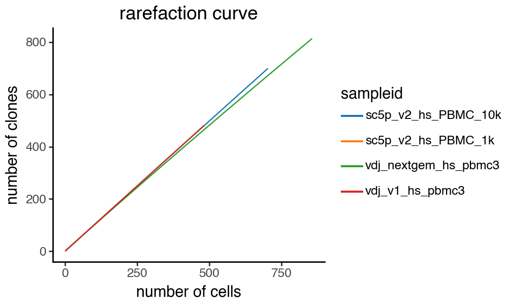
tl.clone_rarefaction and pl.clone_rarefaction
We can use pl.clone_rarefaction to generate rarefaction curves for the clones. tl.clone_rarefaction will populate the .uns slot with the results. groupby option must be specified. In this case, I decided to group by sample. The function will only work on an AnnData object and not a Dandelion object.
[18]:
ddl.pl.clone_rarefaction(adata, color="sampleid")
removing due to zero counts:
Calculating rarefaction curve : 100%|██████████| 4/4 [00:00<00:00, 11.45it/s]
ddl.tl.clone_diversity
tl.clone_diversity allows for calculation of diversity measures such as Chao1, Shannon Entropy and Gini indices.
While the function can work on both AnnData and Dandelion objects, the methods for gini index calculation will only work on a Dandelion object as it requires access to the network.
For Gini indices, we provide several types of measures, inspired by bulk BCRseq analysis methods from [Bashford-Rogers2013]:
The following two indices are returned with metric="clone_network".
network cluster/clone size Gini index
In a contracted BCR network (where identical BCRs are collapsed into the same node/vertex), disparity in the distribution should be correlated to the amount of mutation events i.e. larger networks should indicate more mutation events and smaller networks should indicate lesser mutation events.
network vertex/node size Gini index
In the same contracted network, we can count the number of merged/contracted nodes; nodes with higher count numbers indicate more clonal expansion. Thus, disparity in the distribution of count numbers (referred to as vertex size) should be correlated to the overall clonality i.e. clones with larger vertex sizes are more monoclonal and clones with smaller vertex sizes are more polyclonal.
Therefore, a Gini index of 1 on either measures repesents perfect inequality (i.e. monoclonal and highly mutated) and a value of 0 represents perfect equality (i.e. polyclonal and unmutated).
Note
However, there are a few limitations/challenges that comes with single-cell data:
In the process of contracting the network, we discard the single-cell level information.
Contraction of network is very slow, particularly when there is a lot of clonally-related cells.
For the full implementation and interpretation of both measures, although more evident with cluster/clone size, it requires the BCR repertoire to be reasonably/deeply sampled and we know that this is currently limited by the low recovery from single cell data with current technologies.
Therefore, we implement a few work around options, and ‘experimental’ options below, to try and circumvent these issues.
Firstly, as a work around for (C), the cluster size gini index can be calculated before or after network contraction. If performing before network contraction (default), it will be calculated based on the size of subgraphs of connected components in the main graph. This will retain the single-cell information and should appropriately show the distribution of the data. If performing after network contraction, the calculation is performed after network contraction, achieving the same effect as the
method for bulk BCR-seq as described above. This option can be toggled by use_contracted and only applies to network cluster size gini index calculation.
clone centrality Gini index -
metric="clone_centrality"
Node/vertex closeness centrality indicates how tightly packed clones are (more clonally related) and thus the distribution of the number of cells connected in each clone informs on whether clones in general are more monoclonal or polyclonal.
clone degree Gini index -
metric="clone_degree"
Node/vertex degree indicates how many cells are connected to an individual cell, another indication of how clonally related cells are. However, this would also highlight cells that are in the middle of large networks but are not necessarily within clonally expanded regions (e.g. intermediate connecting cells within the minimum spanning tree).
clone size Gini index -
metric="clone_size"
This is not to be confused with the network cluster size gini index calculation above as this doesn’t rely on the network, although the values should be similar. This is just a simple implementation based on the data frame for the relevant clone_id column. By default, this metric is also returned when running metric=clone_centrality or metric=clone_degree.
Note
For (I) and (II), we can specify expanded_only option to compute the statistic for all clones or expanded only clones. Unlike options (I) and (II), the current calculation for (III) and (IV) is largely influenced by the amount of expanded clones i.e. clones with at least 2 cells, and not affected by the number of singleton clones because singleton clones will have a value of 0 regardless.
The diversity functions also have the option to perform downsampling to a fixed number of cells, or to the smallest sample size specified via groupby (default) so that sample sizes are even when comparing between groups.
if return_table=True, a data frame is returned; otherwise, the value gets added to the AnnData.obs or Dandelion.metadata accordingly.
[19]:
sc.settings.verbosity = 1  # it gets very noisy
ddl.tl.clone_diversity(
    vdj, groupby="sample_id", method="gini", metric="clone_network"
)
ddl.tl.clone_diversity(
    vdj, groupby="sample_id", method="gini", metric="clone_centrality"
)
ddl.tl.transfer(adata, vdj)
[20]:
ddl.pl.clone_network(
    adata,
    color=[
        "clone_network_cluster_size_gini",
        "clone_network_vertex_size_gini",
        "clone_size_gini",
        "clone_centrality_gini",
    ],
    ncols=2,
    size=20,
)
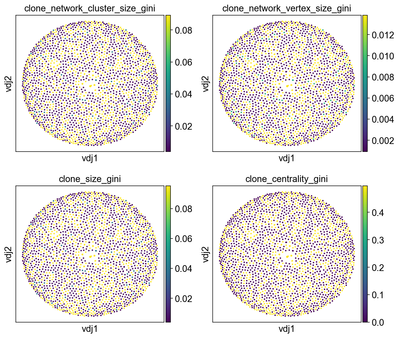
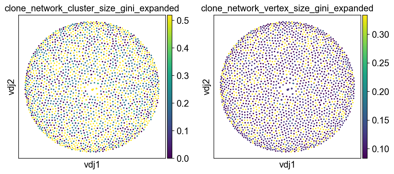
With these particular samples, because there is not many expanded clones in general, the gini indices are quite low when calculated within each sample. We can re-run it by specifying expanded_only = True to only factor in expanded clones. We also specify the key_added option to create a new column instead of writing over the original columns.
[21]:
ddl.tl.clone_diversity(
    vdj,
    groupby="sample_id",
    method="gini",
    metric="clone_network",
    expanded_only=True,
    key_added=[
        "clone_network_cluster_size_gini_expanded",
        "clone_network_vertex_size_gini_expanded",
    ],
)
ddl.tl.transfer(adata, vdj)
[22]:
ddl.pl.clone_network(
    adata,
    color=[
        "clone_network_cluster_size_gini_expanded",
        "clone_network_vertex_size_gini_expanded",
    ],
    ncols=2,
    size=20,
)
We can also choose not to update the metadata to return a pandas dataframe.
[23]:
gini = ddl.tl.clone_diversity(
    vdj, groupby="sample_id", method="gini", return_table=True
)
gini
[23]:
| clone_network_cluster_size_gini | clone_network_vertex_size_gini | |
|---|---|---|
| sc5p_v2_hs_PBMC_10k | 0.006902 | 0.000925 |
| sc5p_v2_hs_PBMC_1k | 0.040145 | 0.009132 |
| vdj_v1_hs_pbmc3 | 0.003976 | 0.001328 |
| vdj_nextgem_hs_pbmc3 | 0.089320 | 0.013850 |
[24]:
gini2 = ddl.tl.clone_diversity(
    vdj,
    groupby="sample_id",
    method="gini",
    return_table=True,
    expanded_only=True,
    key_added=[
        "clone_network_cluster_size_gini_expanded",
        "clone_network_vertex_size_gini_expanded",
    ],
)
gini2
[24]:
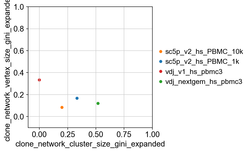
| clone_network_cluster_size_gini_expanded | clone_network_vertex_size_gini_expanded | |
|---|---|---|
| sc5p_v2_hs_PBMC_10k | 0.200000 | 0.083333 |
| sc5p_v2_hs_PBMC_1k | 0.333333 | 0.166667 |
| vdj_v1_hs_pbmc3 | 0.000000 | 0.333333 |
| vdj_nextgem_hs_pbmc3 | 0.519054 | 0.119692 |
[25]:
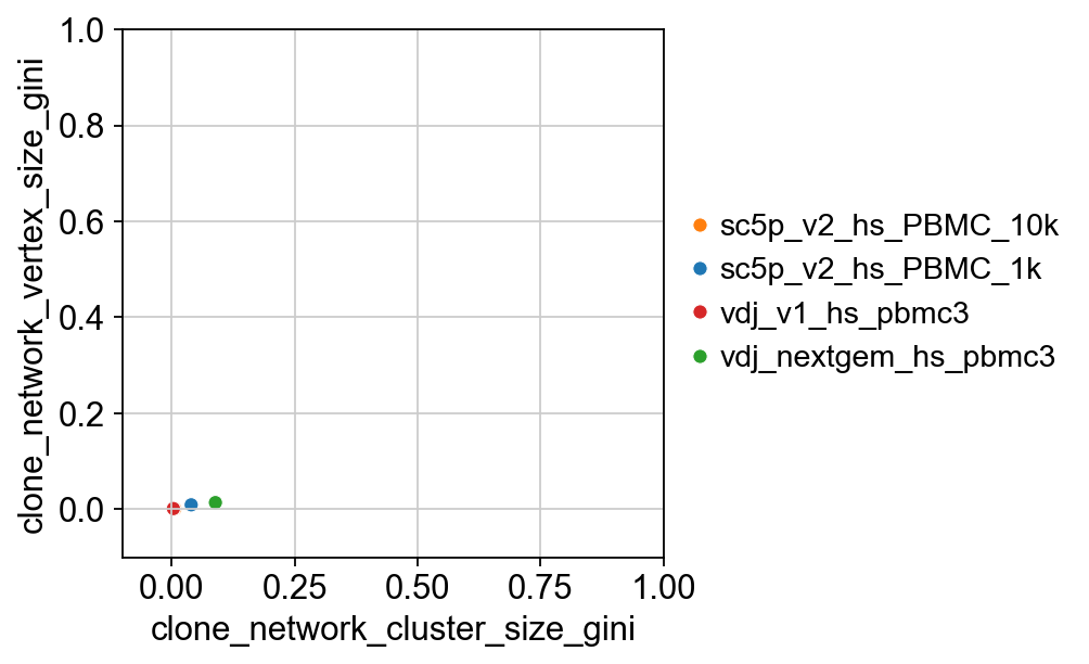
import seaborn as sns
import matplotlib.pyplot as plt

p = sns.scatterplot(
    x="clone_network_cluster_size_gini",
    y="clone_network_vertex_size_gini",
    data=gini,
    hue=gini.index,
    palette=dict(
        zip(adata.obs["sampleid"].cat.categories, adata.uns["sampleid_colors"])
    ),
)
p.set(ylim=(-0.1, 1), xlim=(-0.1, 1))
plt.legend(bbox_to_anchor=(1, 0.5), loc="center left", frameon=False)
p
[25]:
<Axes: xlabel='clone_network_cluster_size_gini', ylabel='clone_network_vertex_size_gini'>
[26]:
p2 = sns.scatterplot(
    x="clone_network_cluster_size_gini_expanded",
    y="clone_network_vertex_size_gini_expanded",
    data=gini2,
    hue=gini2.index,
    palette=dict(
        zip(adata.obs["sampleid"].cat.categories, adata.uns["sampleid_colors"])
    ),
)
p2.set(ylim=(-0.1, 1), xlim=(-0.1, 1))
plt.legend(bbox_to_anchor=(1, 0.5), loc="center left", frameon=False)
p2
[26]:
<Axes: xlabel='clone_network_cluster_size_gini_expanded', ylabel='clone_network_vertex_size_gini_expanded'>
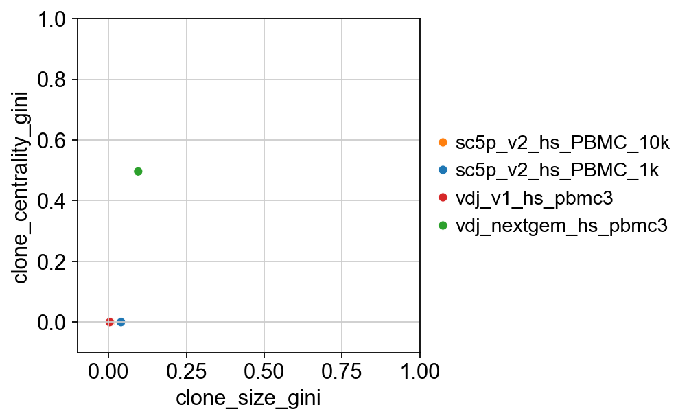
We can also visualise what the results for the clone centrality gini indices.
[27]:
gini = ddl.tl.clone_diversity(
    vdj,
    groupby="sample_id",
    method="gini",
    metric="clone_centrality",
    return_table=True,
)
gini
[27]:
| clone_size_gini | clone_centrality_gini | |
|---|---|---|
| sc5p_v2_hs_PBMC_10k | 0.006902 | 0.000000 |
| sc5p_v2_hs_PBMC_1k | 0.040145 | 0.000000 |
| vdj_v1_hs_pbmc3 | 0.003976 | 0.000000 |
| vdj_nextgem_hs_pbmc3 | 0.095265 | 0.496552 |
[28]:
# not a great example because there's only 1 big clone in 1 sample.
p = sns.scatterplot(
    x="clone_size_gini",
    y="clone_centrality_gini",
    data=gini,
    hue=gini.index,
    palette=dict(
        zip(adata.obs["sampleid"].cat.categories, adata.uns["sampleid_colors"])
    ),
)
p.set(ylim=(-0.1, 1), xlim=(-0.1, 1))
plt.legend(bbox_to_anchor=(1, 0.5), loc="center left", frameon=False)
p
[28]:
<Axes: xlabel='clone_size_gini', ylabel='clone_centrality_gini'>
Chao1 is an estimator based on abundance
[29]:
ddl.tl.clone_diversity(
    vdj, groupby="sample_id", method="chao1", return_table=True
)
[29]:
| clone_size_chao1 | |
|---|---|
| sc5p_v2_hs_PBMC_10k | 51482.600000 |
| sc5p_v2_hs_PBMC_1k | 853.000000 |
| vdj_v1_hs_pbmc3 | 62876.000000 |
| vdj_nextgem_hs_pbmc3 | 13798.538462 |
For Shannon Entropy, we can calculate a normalized (inspired by scirpy’s function) and non-normalized value.
[30]:
ddl.tl.clone_diversity(
    vdj, groupby="sample_id", method="shannon", return_table=True
)
[30]:
| clone_size_normalized_shannon | |
|---|---|
| sc5p_v2_hs_PBMC_10k | 0.999676 |
| sc5p_v2_hs_PBMC_1k | 0.997607 |
| vdj_v1_hs_pbmc3 | 0.999877 |
| vdj_nextgem_hs_pbmc3 | 0.974769 |
[31]:
ddl.tl.clone_diversity(
    vdj,
    groupby="sample_id",
    method="shannon",
    update_obs_meta=False,
    normalize=False,
)
That sums it up for now! Let me know if you have any ideas at [z.tuong@uq.edu.au] and I can try and see if i can implement it or we can work something out to collaborate on!
[ ]: