Visualizing V(D)J data
Integration with scanpy
Now that we have both 1) a pre-processed V(D)J data in Dandelion object and 2) matching AnnData object, we can start finding clones and ‘integrate’ the results. All the V(D)J (AIRR) analyses files can be saved as .tsv format so that it can be used in other tools like immcantation, immunoarch, vdjtools, etc.
The results can also be ported into the AnnData object for access to more plotting functions provided through scanpy [Wolf2018].
Import modules
[1]:
import os
import dandelion as ddl

ddl.logging.print_header()
/opt/homebrew/Caskroom/miniforge/base/envs/dandelion/lib/python3.11/site-packages/anndata/utils.py:429: FutureWarning: Importing read_csv from `anndata` is deprecated. Import anndata.io.read_csv instead.
/opt/homebrew/Caskroom/miniforge/base/envs/dandelion/lib/python3.11/site-packages/anndata/utils.py:429: FutureWarning: Importing read_excel from `anndata` is deprecated. Import anndata.io.read_excel instead.
/opt/homebrew/Caskroom/miniforge/base/envs/dandelion/lib/python3.11/site-packages/anndata/utils.py:429: FutureWarning: Importing read_hdf from `anndata` is deprecated. Import anndata.io.read_hdf instead.
/opt/homebrew/Caskroom/miniforge/base/envs/dandelion/lib/python3.11/site-packages/anndata/utils.py:429: FutureWarning: Importing read_loom from `anndata` is deprecated. Import anndata.io.read_loom instead.
/opt/homebrew/Caskroom/miniforge/base/envs/dandelion/lib/python3.11/site-packages/anndata/utils.py:429: FutureWarning: Importing read_mtx from `anndata` is deprecated. Import anndata.io.read_mtx instead.
/opt/homebrew/Caskroom/miniforge/base/envs/dandelion/lib/python3.11/site-packages/anndata/utils.py:429: FutureWarning: Importing read_text from `anndata` is deprecated. Import anndata.io.read_text instead.
/opt/homebrew/Caskroom/miniforge/base/envs/dandelion/lib/python3.11/site-packages/anndata/utils.py:429: FutureWarning: Importing read_umi_tools from `anndata` is deprecated. Import anndata.io.read_umi_tools instead.
dandelion==0.5.5.dev16 pandas==2.2.3 numpy==2.1.3 matplotlib==3.10.1 networkx==3.4.2 scipy==1.15.2
/opt/homebrew/Caskroom/miniforge/base/envs/dandelion/lib/python3.11/site-packages/nxviz/__init__.py:33: UserWarning:
nxviz has a new API! Version 0.7.4 onwards, the old class-based API is being
deprecated in favour of a new API focused on advancing a grammar of network
graphics. If your plotting code depends on the old API, please consider
pinning nxviz at version 0.7.4, as the new API will break your old code.

To check out the new API, please head over to the docs at
https://ericmjl.github.io/nxviz/ to learn more. We hope you enjoy using it!

(This deprecation message will go away in version 1.0.)
[2]:
# change directory to somewhere more workable
os.chdir(os.path.expanduser("~/Downloads/dandelion_tutorial/"))
# I'm importing scanpy here to make use of its logging module.
import scanpy as sc

sc.settings.verbosity = 3
import warnings

warnings.filterwarnings("ignore")
sc.logging.print_header()
scanpy==1.10.3 anndata==0.11.3 umap==0.5.7 numpy==2.1.3 scipy==1.15.2 pandas==2.2.3 scikit-learn==1.6.1 statsmodels==0.14.4 igraph==0.11.8 pynndescent==0.5.13
Read in the previously saved files
I will work with the same example from the previous section since I have the AnnData object saved and vdj table filtered.
[3]:
adata = sc.read_h5ad("adata.h5ad")
[4]:
vdj = ddl.read_h5ddl("dandelion_results_simplified.h5ddl")
vdj
[4]:
Dandelion class object with n_obs = 2112 and n_contigs = 5052
    data: 'sequence_id', 'sequence', 'rev_comp', 'productive', 'v_call', 'd_call', 'j_call', 'sequence_alignment', 'germline_alignment', 'junction', 'junction_aa', 'v_cigar', 'd_cigar', 'j_cigar', 'stop_codon', 'vj_in_frame', 'locus', 'c_call', 'junction_length', 'np1_length', 'np2_length', 'v_sequence_start', 'v_sequence_end', 'v_germline_start', 'v_germline_end', 'd_sequence_start', 'd_sequence_end', 'd_germline_start', 'd_germline_end', 'j_sequence_start', 'j_sequence_end', 'j_germline_start', 'j_germline_end', 'v_score', 'v_identity', 'v_support', 'd_score', 'd_identity', 'd_support', 'j_score', 'j_identity', 'j_support', 'fwr1', 'fwr2', 'fwr3', 'fwr4', 'cdr1', 'cdr2', 'cdr3', 'cell_id', 'consensus_count', 'umi_count', 'v_call_10x', 'd_call_10x', 'j_call_10x', 'junction_10x', 'junction_10x_aa', 'j_support_igblastn', 'j_score_igblastn', 'j_call_igblastn', 'j_call_blastn', 'j_identity_blastn', 'j_alignment_length_blastn', 'j_number_of_mismatches_blastn', 'j_number_of_gap_openings_blastn', 'j_sequence_start_blastn', 'j_sequence_end_blastn', 'j_germline_start_blastn', 'j_germline_end_blastn', 'j_support_blastn', 'j_score_blastn', 'j_sequence_alignment_blastn', 'j_germline_alignment_blastn', 'j_source', 'd_support_igblastn', 'd_score_igblastn', 'd_call_igblastn', 'd_call_blastn', 'd_identity_blastn', 'd_alignment_length_blastn', 'd_number_of_mismatches_blastn', 'd_number_of_gap_openings_blastn', 'd_sequence_start_blastn', 'd_sequence_end_blastn', 'd_germline_start_blastn', 'd_germline_end_blastn', 'd_support_blastn', 'd_score_blastn', 'd_sequence_alignment_blastn', 'd_germline_alignment_blastn', 'd_source', 'v_call_genotyped', 'germline_alignment_d_mask', 'sample_id', 'c_sequence_alignment', 'c_germline_alignment', 'c_sequence_start', 'c_sequence_end', 'c_score', 'c_identity', 'c_call_10x', 'junction_aa_length', 'fwr1_aa', 'fwr2_aa', 'fwr3_aa', 'fwr4_aa', 'cdr1_aa', 'cdr2_aa', 'cdr3_aa', 'sequence_alignment_aa', 'v_sequence_alignment_aa', 'd_sequence_alignment_aa', 'j_sequence_alignment_aa', 'complete_vdj', 'j_call_multimappers', 'j_call_multiplicity', 'j_call_sequence_start_multimappers', 'j_call_sequence_end_multimappers', 'j_call_support_multimappers', 'mu_count', 'ambiguous', 'extra', 'rearrangement_status', 'clone_id', 'changeo_clone_id'
    metadata: 'clone_id', 'clone_id_by_size', 'sample_id', 'locus_VDJ', 'locus_VJ', 'productive_VDJ', 'productive_VJ', 'v_call_genotyped_VDJ', 'd_call_VDJ', 'j_call_VDJ', 'v_call_genotyped_VJ', 'j_call_VJ', 'c_call_VDJ', 'c_call_VJ', 'junction_VDJ', 'junction_VJ', 'junction_aa_VDJ', 'junction_aa_VJ', 'v_call_genotyped_B_VDJ', 'd_call_B_VDJ', 'j_call_B_VDJ', 'v_call_genotyped_B_VJ', 'j_call_B_VJ', 'c_call_B_VDJ', 'c_call_B_VJ', 'productive_B_VDJ', 'productive_B_VJ', 'umi_count_B_VDJ', 'umi_count_B_VJ', 'v_call_VDJ_main', 'v_call_VJ_main', 'd_call_VDJ_main', 'j_call_VDJ_main', 'j_call_VJ_main', 'c_call_VDJ_main', 'c_call_VJ_main', 'v_call_B_VDJ_main', 'd_call_B_VDJ_main', 'j_call_B_VDJ_main', 'v_call_B_VJ_main', 'j_call_B_VJ_main', 'isotype', 'isotype_status', 'locus_status', 'chain_status', 'rearrangement_status_VDJ', 'rearrangement_status_VJ', 'changeo_clone_id'
    layout: layout for 2112 vertices, layout for 71 vertices
    graph: networkx graph of 2112 vertices, networkx graph of 71 vertices
tl.transfer
To proceed, we first need to initialise the AnnData object with our network. This is done by using the tool function tl.transfer.
[5]:
ddl.tl.transfer(adata, vdj)  # this will include singletons.
adata
Transferring network
converting matrices
Updating anndata slots
 finished: updated `.obs` with `.metadata`
added to `.uns['neighbors']` and `.uns['clone_id']`
and `.obsp`
   'distances', clonotype-weighted adjacency matrix
   'connectivities', clonotype-weighted adjacency matrix (0:00:09)
[5]:
AnnData object with n_obs × n_vars = 23715 × 1400
    obs: 'sampleid', 'batch', 'n_genes', 'n_genes_by_counts', 'total_counts', 'total_counts_mt', 'pct_counts_mt', 'gmm_pct_count_clusters_keep', 'scrublet_score', 'is_doublet', 'filter_rna', 'has_contig', 'sample_id', 'locus_VDJ', 'locus_VJ', 'productive_VDJ', 'productive_VJ', 'v_call_genotyped_VDJ', 'd_call_VDJ', 'j_call_VDJ', 'v_call_genotyped_VJ', 'j_call_VJ', 'c_call_VDJ', 'c_call_VJ', 'junction_VDJ', 'junction_VJ', 'junction_aa_VDJ', 'junction_aa_VJ', 'v_call_genotyped_B_VDJ', 'd_call_B_VDJ', 'j_call_B_VDJ', 'v_call_genotyped_B_VJ', 'j_call_B_VJ', 'c_call_B_VDJ', 'c_call_B_VJ', 'productive_B_VDJ', 'productive_B_VJ', 'umi_count_B_VDJ', 'umi_count_B_VJ', 'v_call_VDJ_main', 'v_call_VJ_main', 'd_call_VDJ_main', 'j_call_VDJ_main', 'j_call_VJ_main', 'c_call_VDJ_main', 'c_call_VJ_main', 'v_call_B_VDJ_main', 'd_call_B_VDJ_main', 'j_call_B_VDJ_main', 'v_call_B_VJ_main', 'j_call_B_VJ_main', 'isotype', 'isotype_status', 'locus_status', 'chain_status', 'rearrangement_status_VDJ', 'rearrangement_status_VJ', 'leiden', 'clone_id', 'clone_id_by_size', 'changeo_clone_id'
    var: 'feature_types', 'genome', 'pattern', 'read', 'sequence', 'gene_ids-0', 'gene_ids-1', 'gene_ids-2', 'gene_ids-3', 'n_cells', 'highly_variable', 'means', 'dispersions', 'dispersions_norm', 'mean', 'std'
    uns: 'chain_status_colors', 'hvg', 'leiden', 'leiden_colors', 'log1p', 'neighbors', 'pca', 'umap', 'rna_neighbors', 'clone_id'
    obsm: 'X_pca', 'X_umap', 'X_vdj'
    varm: 'PCs'
    obsp: 'connectivities', 'distances', 'rna_connectivities', 'rna_distances', 'vdj_connectivities', 'vdj_distances'
To show only expanded clones, specify expanded_only=True
[6]:
adata2 = adata.copy()
ddl.tl.transfer(adata2, vdj, expanded_only=True)
adata2
Transferring network
converting matrices
Updating anndata slots
 finished: updated `.obs` with `.metadata`
added to `.uns['neighbors']` and `.uns['clone_id']`
and `.obsp`
   'distances', clonotype-weighted adjacency matrix
   'connectivities', clonotype-weighted adjacency matrix (0:00:09)
[6]:
AnnData object with n_obs × n_vars = 23715 × 1400
    obs: 'sampleid', 'batch', 'n_genes', 'n_genes_by_counts', 'total_counts', 'total_counts_mt', 'pct_counts_mt', 'gmm_pct_count_clusters_keep', 'scrublet_score', 'is_doublet', 'filter_rna', 'has_contig', 'sample_id', 'locus_VDJ', 'locus_VJ', 'productive_VDJ', 'productive_VJ', 'v_call_genotyped_VDJ', 'd_call_VDJ', 'j_call_VDJ', 'v_call_genotyped_VJ', 'j_call_VJ', 'c_call_VDJ', 'c_call_VJ', 'junction_VDJ', 'junction_VJ', 'junction_aa_VDJ', 'junction_aa_VJ', 'v_call_genotyped_B_VDJ', 'd_call_B_VDJ', 'j_call_B_VDJ', 'v_call_genotyped_B_VJ', 'j_call_B_VJ', 'c_call_B_VDJ', 'c_call_B_VJ', 'productive_B_VDJ', 'productive_B_VJ', 'umi_count_B_VDJ', 'umi_count_B_VJ', 'v_call_VDJ_main', 'v_call_VJ_main', 'd_call_VDJ_main', 'j_call_VDJ_main', 'j_call_VJ_main', 'c_call_VDJ_main', 'c_call_VJ_main', 'v_call_B_VDJ_main', 'd_call_B_VDJ_main', 'j_call_B_VDJ_main', 'v_call_B_VJ_main', 'j_call_B_VJ_main', 'isotype', 'isotype_status', 'locus_status', 'chain_status', 'rearrangement_status_VDJ', 'rearrangement_status_VJ', 'leiden', 'clone_id', 'clone_id_by_size', 'changeo_clone_id'
    var: 'feature_types', 'genome', 'pattern', 'read', 'sequence', 'gene_ids-0', 'gene_ids-1', 'gene_ids-2', 'gene_ids-3', 'n_cells', 'highly_variable', 'means', 'dispersions', 'dispersions_norm', 'mean', 'std'
    uns: 'chain_status_colors', 'hvg', 'leiden', 'leiden_colors', 'log1p', 'neighbors', 'pca', 'umap', 'rna_neighbors', 'clone_id'
    obsm: 'X_pca', 'X_umap', 'X_vdj'
    varm: 'PCs'
    obsp: 'connectivities', 'distances', 'rna_connectivities', 'rna_distances', 'vdj_connectivities', 'vdj_distances'
Note
If a column with the same name between Dandelion.metadata and AnnData.obs already exists, tl.transfer will not overwrite the column in the AnnData object. This can be toggled to overwrite all with overwrite=True or overwrite=["column_name1", "column_name2"] if only some columns are to be overwritten.
You can see that AnnData object now contains a couple more columns in the .obs slot, corresponding to the metadata that is returned after tl.generate_network, and newly populated .obsm and .obsp slots. The original RNA connectivities and distances are now added into the .obsp slot as well.
Plotting in scanpy
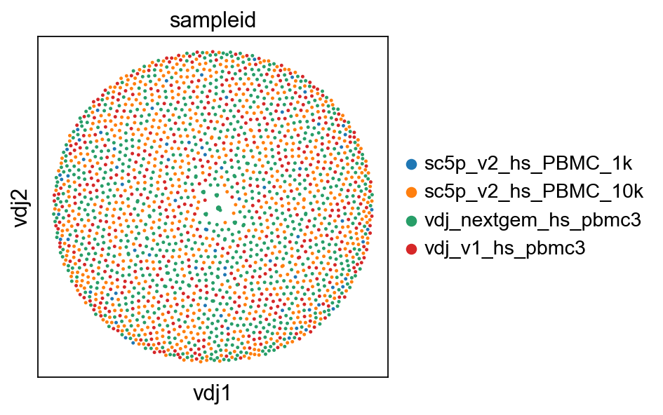
pl.clone_network
So now, basically we can plot in scanpy with their plotting modules. I’ve included a plotting function in dandelion, pl.clone_network, which is really just a wrapper of their pl.embedding module.
[7]:
sc.set_figure_params(figsize=[4, 4])
ddl.pl.clone_network(adata, color=["sampleid"], edges_width=1, size=20)
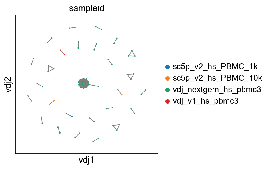
# show where clones/clonotypes have more than 1 cell
ddl.pl.clone_network(adata2, color=["sampleid"], edges_width=1, size=20)
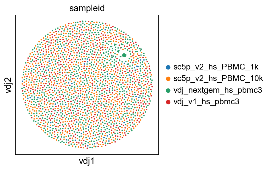
Note
if you prefer the original (modified) Fruchterman-Reingold layout, you can generate the layout with layout_method="mod_fr". Just note that this is significantly slower. Although the X and Y axes (vdj1 and vdj2) are arbitrary, the mod_fr layout seems to produce more pronounced repulsion between clusters, so something to keep in mind for when trying to work with a lot of cells/clusters as it can lead to really pretty (or ugly) plots.
[8]:
# making a copy of both adata and vdj
vdj3 = vdj.copy()
adata3 = adata.copy()
# recompute layout with original method
ddl.tl.generate_network(vdj3, layout_method="mod_fr")
ddl.tl.transfer(adata3, vdj3)
# also for > 1 cells
adata4 = adata3.copy()
ddl.tl.transfer(adata4, vdj3, expanded_only=True)
# visualise
ddl.pl.clone_network(adata3, color=["sampleid"], edges_width=1, size=20)
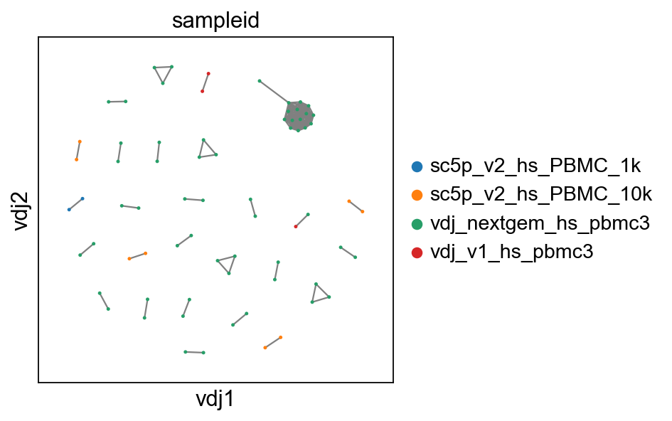
# show where clones/clonotypes have more than 1 cell
ddl.pl.clone_network(adata4, color=["sampleid"], edges_width=1, size=20)
Generating network layout from pre-computed network
Computing network layout
Computing expanded network layout
 finished: Updated Dandelion object:
   'data', contig-indexed AIRR table
   'metadata', cell-indexed observations table
   'layout', graph layout
   'graph', network constructed from distance matrices of VDJ- and VJ- chains (0:00:05)
Transferring network
converting matrices
Updating anndata slots
 finished: updated `.obs` with `.metadata`
added to `.uns['neighbors']` and `.uns['clone_id']`
and `.obsp`
   'distances', clonotype-weighted adjacency matrix
   'connectivities', clonotype-weighted adjacency matrix (0:00:10)
Transferring network
converting matrices
Updating anndata slots
 finished: updated `.obs` with `.metadata`
added to `.uns['neighbors']` and `.uns['clone_id']`
and `.obsp`
   'distances', clonotype-weighted adjacency matrix
   'connectivities', clonotype-weighted adjacency matrix (0:00:10)
tl.extract_edge_weights
dandelion provides an edge weight extractor tool tl.extract_edge_weights to retrieve the edge weights that can be used to specify the edge widths according to weight/distance.
[9]:
# To illustrate this, first recompute the graph by specifying a minimum size
vdjx = vdj.copy()
adatax = adata.copy()
ddl.tl.generate_network(
    vdjx, min_size=3
)  # second graph will only contain clones/clonotypes with >= 3 cells
ddl.tl.transfer(adatax, vdjx, expanded_only=True)

edgeweights = [
    1 / (e + 1) for e in ddl.tl.extract_edge_weights(vdjx)
]  # invert and add 1 to each edge weight (e) so that distance of 0 becomes the thickest edge
# therefore, the thicker the line, the shorter the edit distance.
ddl.pl.clone_network(
    adatax,
    color=["isotype_status"],
    legend_fontoutline=3,
    edges_width=edgeweights,
    size=50,
)
Generating network
Setting up data: 4424it [00:00, 6077.79it/s]
Calculating distances : 100%|██████████| 2313/2313 [00:00<00:00, 11877.85it/s]
Aggregating distances : 100%|██████████| 5/5 [00:00<00:00, 113.89it/s]
Sorting into clusters : 100%|██████████| 2313/2313 [00:00<00:00, 4419.08it/s]
Calculating minimum spanning tree : 100%|██████████| 35/35 [00:00<00:00, 1251.38it/s]
Generating edge list : 100%|██████████| 35/35 [00:00<00:00, 4736.12it/s]
Computing overlap : 100%|██████████| 2313/2313 [00:00<00:00, 3780.46it/s]
Adjust overlap : 100%|██████████| 143/143 [00:00<00:00, 4775.10it/s]
Linking edges : 100%|██████████| 2062/2062 [00:00<00:00, 57801.05it/s]
Computing network layout
Computing expanded network layout
 finished: Updated Dandelion object:
   'data', contig-indexed AIRR table
   'metadata', cell-indexed observations table
   'layout', graph layout
   'graph', network constructed from distance matrices of VDJ- and VJ- chains (0:00:05)
Transferring network
converting matrices
Updating anndata slots
 finished: updated `.obs` with `.metadata`
added to `.uns['neighbors']` and `.uns['clone_id']`
and `.obsp`
   'distances', clonotype-weighted adjacency matrix
   'connectivities', clonotype-weighted adjacency matrix (0:00:09)
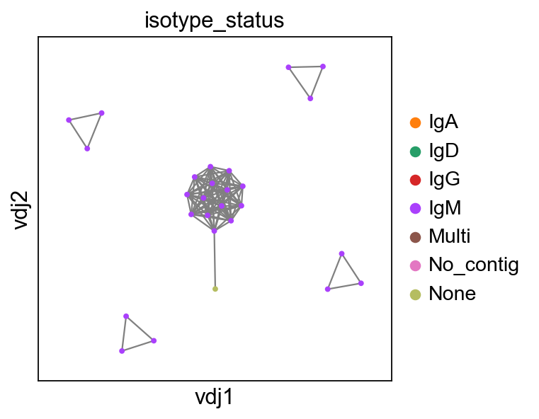
None here means there is no isotype information i.e. no c_call. If No_contig appears, it means there’s no V(D)J information.
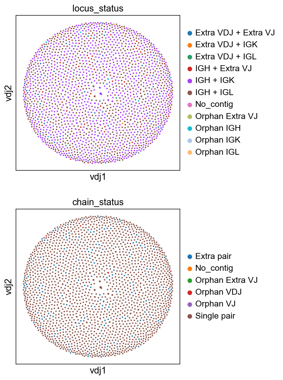
You can interact with pl.clone_network just as how you interact with the rest of the scatterplot modules in scanpy.
[10]:
sc.set_figure_params(figsize=[4, 4.5])
ddl.pl.clone_network(
    adata,
    color=["locus_status", "chain_status"],
    ncols=1,
    legend_fontoutline=3,
    edges_width=1,
    size=20,
)
you should be able to save the adata object and interact with it as per normal.
[11]:
# adata.write("adata.h5ad", compression="gzip")
Calculating size of clones
tl.clone_size
Sometimes it’s useful to evaluate the size of the clone. Here tl.quantify_clone_size does a simple calculation to enable that.
[12]:
ddl.tl.clone_size(vdj)
ddl.tl.transfer(adata, vdj)
Quantifying clone sizes
 finished: Updated Dandelion object:
   'metadata', cell-indexed clone table (0:00:00)
Transferring network
converting matrices
Updating anndata slots
 finished: updated `.obs` with `.metadata`
added to `.uns['neighbors']` and `.uns['clone_id']`
and `.obsp`
   'distances', clonotype-weighted adjacency matrix
   'connectivities', clonotype-weighted adjacency matrix (0:00:09)
[13]:
sc.set_figure_params(figsize=[5, 4.5])
ddl.pl.clone_network(
    adata,
    color=["clone_id_size"],
    legend_fontoutline=3,
    edges_width=1,
    size=20,
    color_map="viridis",
)
sc.pl.umap(adata, color=["clone_id_size"], color_map="viridis")


You can also specify max_size to clip off the calculation at a fixed value.
[14]:
ddl.tl.clone_size(vdj, max_size=3)
ddl.tl.transfer(adata, vdj)
Quantifying clone sizes
 finished: Updated Dandelion object:
   'metadata', cell-indexed clone table (0:00:00)
Transferring network
converting matrices
Updating anndata slots
 finished: updated `.obs` with `.metadata`
added to `.uns['neighbors']` and `.uns['clone_id']`
and `.obsp`
   'distances', clonotype-weighted adjacency matrix
   'connectivities', clonotype-weighted adjacency matrix (0:00:09)
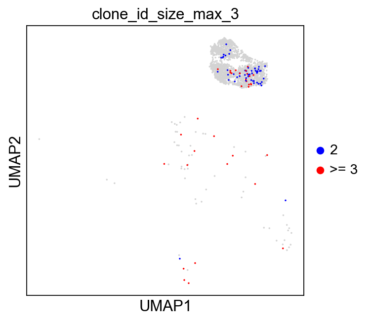
[15]:
sc.set_figure_params(figsize=[4.5, 4.5])
ddl.pl.clone_network(
    adata,
    color=["clone_id_size_max_3"],
    ncols=2,
    legend_fontoutline=3,
    edges_width=1,
    palette=["grey", "blue", "red"],
    size=20,
    na_in_legend=False,
)
sc.pl.umap(
    adata[adata.obs["has_contig"] == "True"],
    color=["clone_id_size_max_3"],
    groups=["2", ">= 3"],
    size=10,
    na_in_legend=False,
)

Additional plotting functions
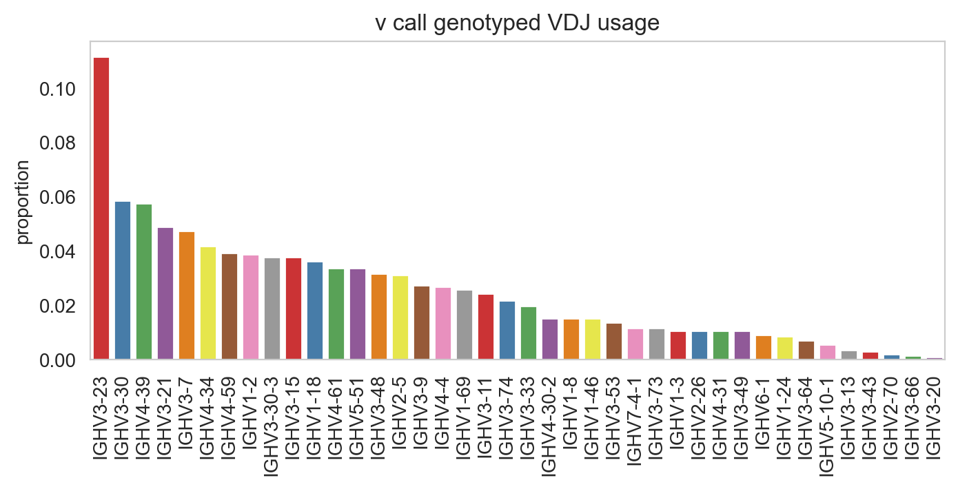
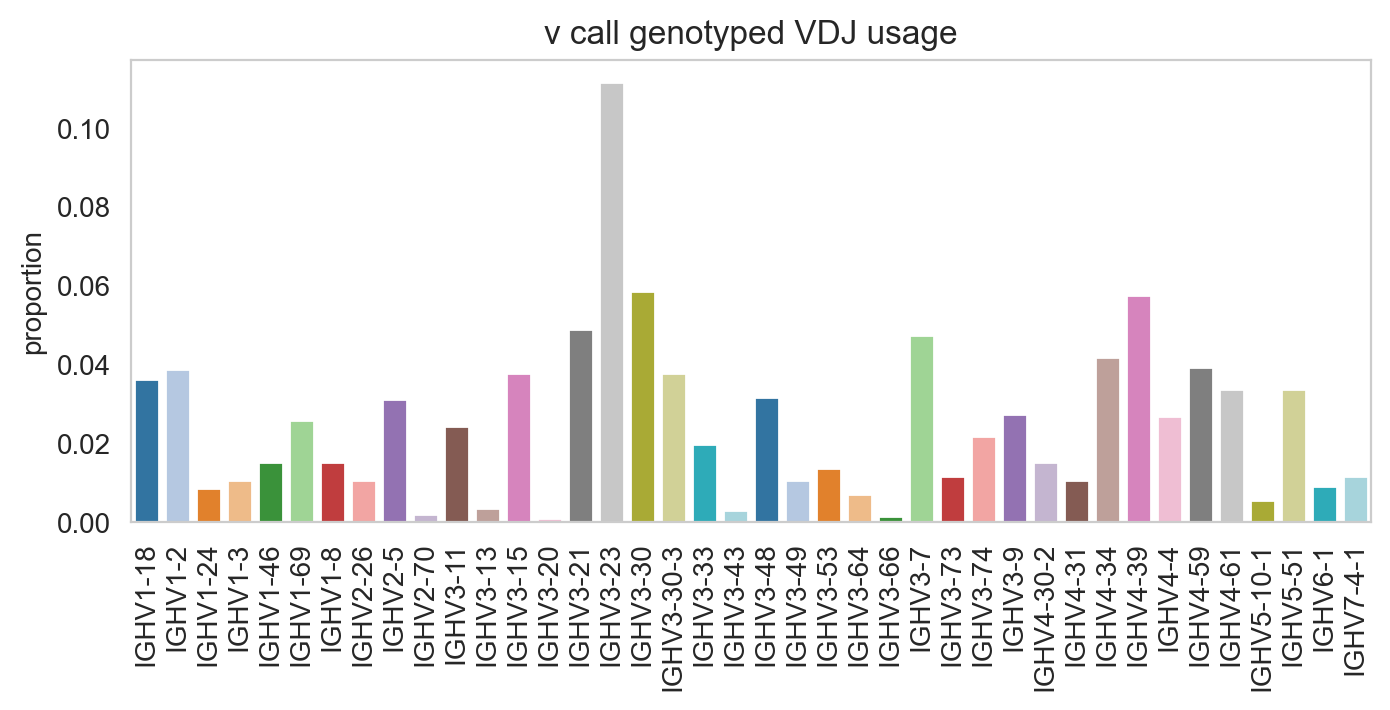
ddl.pl.barplot
pl.barplot is a generic barplot function that will plot items in the metadata slot as a bar plot. This function will also interact with .obs slot if a scanpy object is used in place of Dandelion object. However, if your scanpy object holds a lot of non-B cells, then the plotting will be just be saturated with nan values.
Let’s first slice the Dandelion object to only include cells with at most one heavy chain.
[16]:
vdj_subset = vdj[
    vdj.metadata["chain_status"].isin(["Single pair", "Orphan VDJ"])
]
vdj_subset
[16]:
Dandelion class object with n_obs = 1962 and n_contigs = 4485
    data: 'sequence_id', 'sequence', 'rev_comp', 'productive', 'v_call', 'd_call', 'j_call', 'sequence_alignment', 'germline_alignment', 'junction', 'junction_aa', 'v_cigar', 'd_cigar', 'j_cigar', 'stop_codon', 'vj_in_frame', 'locus', 'c_call', 'junction_length', 'np1_length', 'np2_length', 'v_sequence_start', 'v_sequence_end', 'v_germline_start', 'v_germline_end', 'd_sequence_start', 'd_sequence_end', 'd_germline_start', 'd_germline_end', 'j_sequence_start', 'j_sequence_end', 'j_germline_start', 'j_germline_end', 'v_score', 'v_identity', 'v_support', 'd_score', 'd_identity', 'd_support', 'j_score', 'j_identity', 'j_support', 'fwr1', 'fwr2', 'fwr3', 'fwr4', 'cdr1', 'cdr2', 'cdr3', 'cell_id', 'consensus_count', 'umi_count', 'v_call_10x', 'd_call_10x', 'j_call_10x', 'junction_10x', 'junction_10x_aa', 'j_support_igblastn', 'j_score_igblastn', 'j_call_igblastn', 'j_call_blastn', 'j_identity_blastn', 'j_alignment_length_blastn', 'j_number_of_mismatches_blastn', 'j_number_of_gap_openings_blastn', 'j_sequence_start_blastn', 'j_sequence_end_blastn', 'j_germline_start_blastn', 'j_germline_end_blastn', 'j_support_blastn', 'j_score_blastn', 'j_sequence_alignment_blastn', 'j_germline_alignment_blastn', 'j_source', 'd_support_igblastn', 'd_score_igblastn', 'd_call_igblastn', 'd_call_blastn', 'd_identity_blastn', 'd_alignment_length_blastn', 'd_number_of_mismatches_blastn', 'd_number_of_gap_openings_blastn', 'd_sequence_start_blastn', 'd_sequence_end_blastn', 'd_germline_start_blastn', 'd_germline_end_blastn', 'd_support_blastn', 'd_score_blastn', 'd_sequence_alignment_blastn', 'd_germline_alignment_blastn', 'd_source', 'v_call_genotyped', 'germline_alignment_d_mask', 'sample_id', 'c_sequence_alignment', 'c_germline_alignment', 'c_sequence_start', 'c_sequence_end', 'c_score', 'c_identity', 'c_call_10x', 'junction_aa_length', 'fwr1_aa', 'fwr2_aa', 'fwr3_aa', 'fwr4_aa', 'cdr1_aa', 'cdr2_aa', 'cdr3_aa', 'sequence_alignment_aa', 'v_sequence_alignment_aa', 'd_sequence_alignment_aa', 'j_sequence_alignment_aa', 'complete_vdj', 'j_call_multimappers', 'j_call_multiplicity', 'j_call_sequence_start_multimappers', 'j_call_sequence_end_multimappers', 'j_call_support_multimappers', 'mu_count', 'ambiguous', 'extra', 'rearrangement_status', 'clone_id', 'changeo_clone_id'
    metadata: 'clone_id', 'clone_id_by_size', 'sample_id', 'locus_VDJ', 'locus_VJ', 'productive_VDJ', 'productive_VJ', 'v_call_genotyped_VDJ', 'd_call_VDJ', 'j_call_VDJ', 'v_call_genotyped_VJ', 'j_call_VJ', 'c_call_VDJ', 'c_call_VJ', 'junction_VDJ', 'junction_VJ', 'junction_aa_VDJ', 'junction_aa_VJ', 'v_call_genotyped_B_VDJ', 'd_call_B_VDJ', 'j_call_B_VDJ', 'v_call_genotyped_B_VJ', 'j_call_B_VJ', 'c_call_B_VDJ', 'c_call_B_VJ', 'productive_B_VDJ', 'productive_B_VJ', 'umi_count_B_VDJ', 'umi_count_B_VJ', 'v_call_VDJ_main', 'v_call_VJ_main', 'd_call_VDJ_main', 'j_call_VDJ_main', 'j_call_VJ_main', 'c_call_VDJ_main', 'c_call_VJ_main', 'v_call_B_VDJ_main', 'd_call_B_VDJ_main', 'j_call_B_VDJ_main', 'v_call_B_VJ_main', 'j_call_B_VJ_main', 'isotype', 'isotype_status', 'locus_status', 'chain_status', 'rearrangement_status_VDJ', 'rearrangement_status_VJ', 'changeo_clone_id', 'clone_id_size', 'clone_id_size_max_3'
    layout: layout for 1962 vertices, layout for 71 vertices
    graph: networkx graph of 1962 vertices, networkx graph of 71 vertices
[17]:
import matplotlib as mpl
import matplotlib.pyplot as plt

mpl.rcParams.update(mpl.rcParamsDefault)

ddl.pl.barplot(
    vdj_subset,
    color="v_call_genotyped_VDJ",
)
plt.show()
You can prevent it from sorting by specifying sort_descending = None. Colours can be changed with palette option.
[18]:
ddl.pl.barplot(
    vdj_subset,
    color="v_call_genotyped_VDJ",
    sort_descending=None,
    palette="tab20",
)
plt.show()
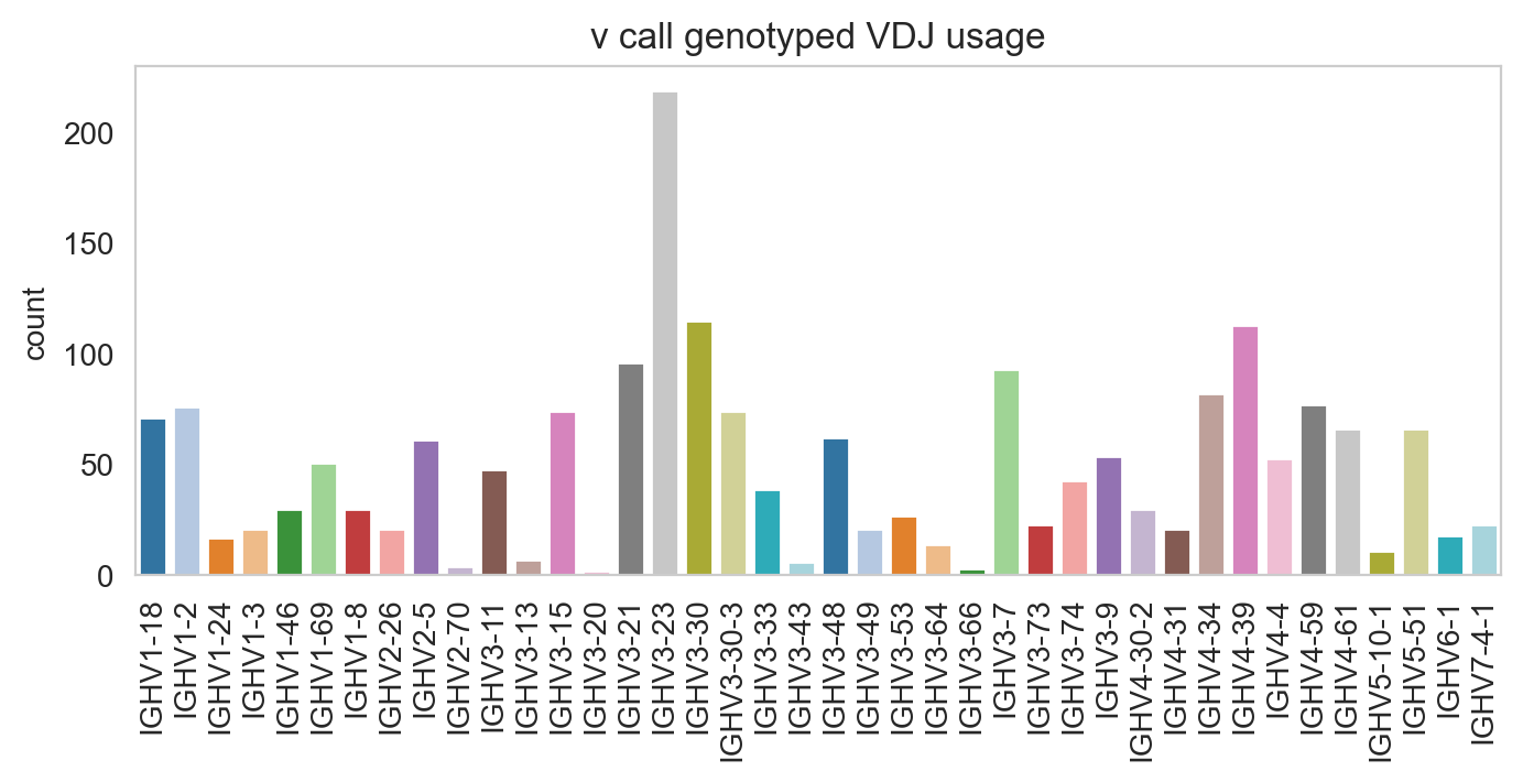
Specifying normalize = False will change the y-axis to counts.
[19]:
ddl.pl.barplot(
    vdj_subset,
    color="v_call_genotyped_VDJ",
    normalize=False,
    sort_descending=None,
    palette="tab20",
)
plt.show()
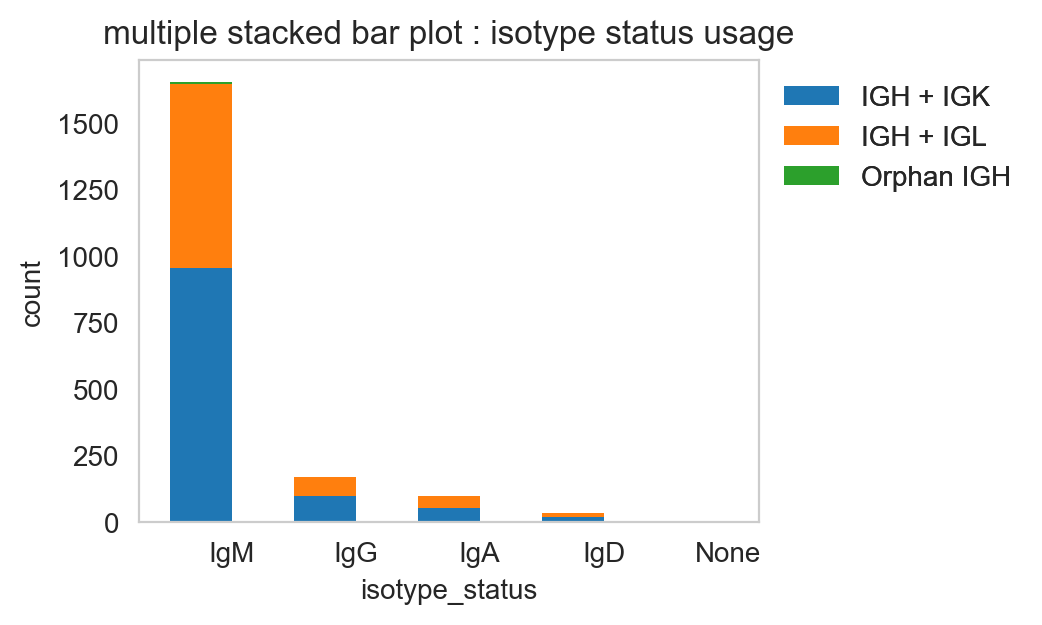
pl.stackedbarplot
pl.stackedbarplot is similar to above but can split between specified groups. Some examples below:
[20]:
ddl.pl.stackedbarplot(
    vdj_subset,
    color="isotype_status",
    groupby="locus_status",
    xtick_rotation=0,
    figsize=(4, 3),
)
plt.legend(bbox_to_anchor=(1, 1), loc="upper left", frameon=False)
plt.show()
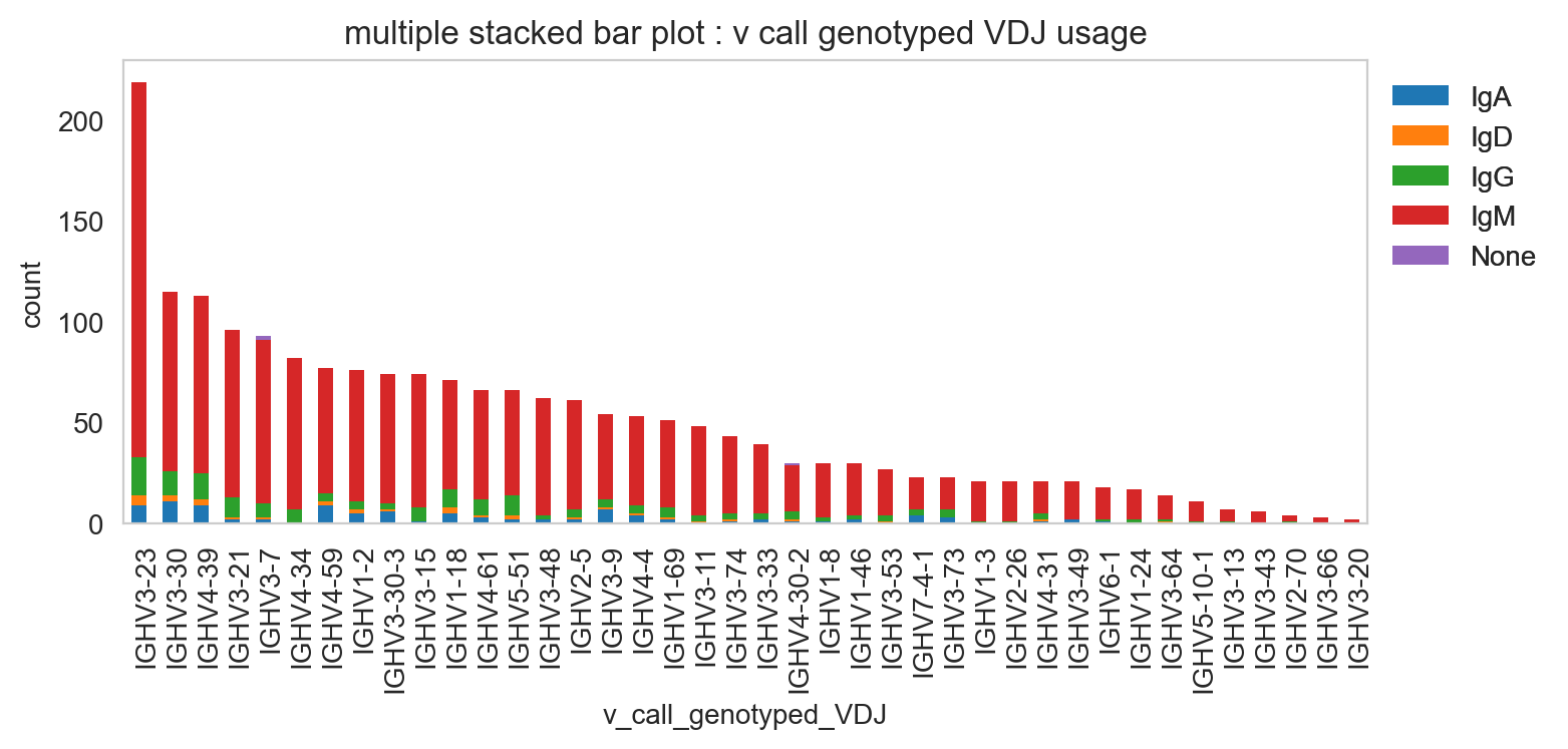
[21]:
ddl.pl.stackedbarplot(
    vdj_subset,
    color="v_call_genotyped_VDJ",
    groupby="isotype_status",
)
plt.legend(bbox_to_anchor=(1, 1), loc="upper left", frameon=False)
plt.show()
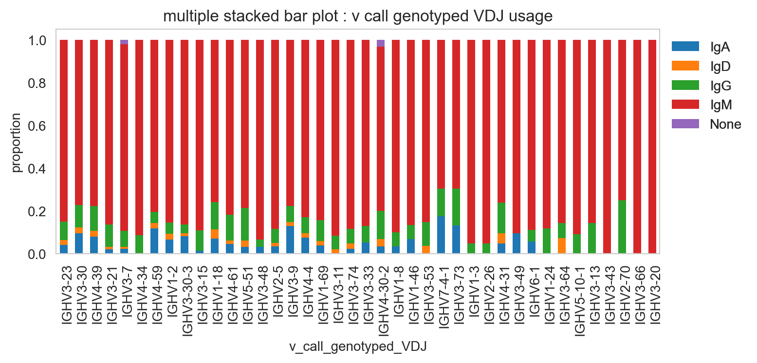
[22]:
ddl.pl.stackedbarplot(
    vdj_subset,
    color="v_call_genotyped_VDJ",
    groupby="isotype_status",
    normalize=True,
)
plt.legend(bbox_to_anchor=(1, 1), loc="upper left", frameon=False)
plt.show()
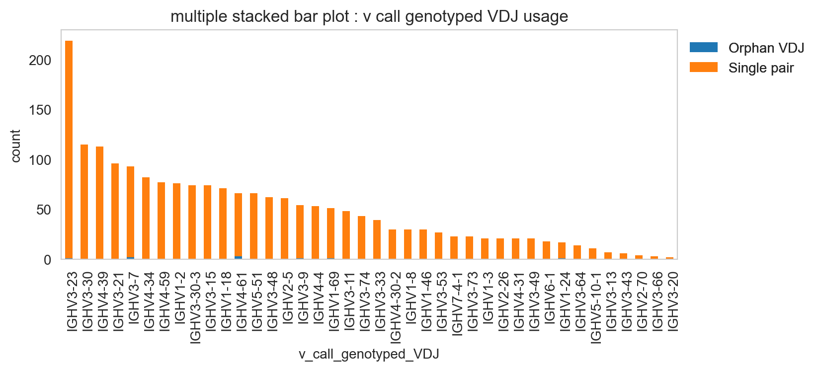
[23]:
ddl.pl.stackedbarplot(
    vdj_subset,
    color="v_call_genotyped_VDJ",
    groupby="chain_status",
)
plt.legend(bbox_to_anchor=(1, 1), loc="upper left", frameon=False)
plt.show()
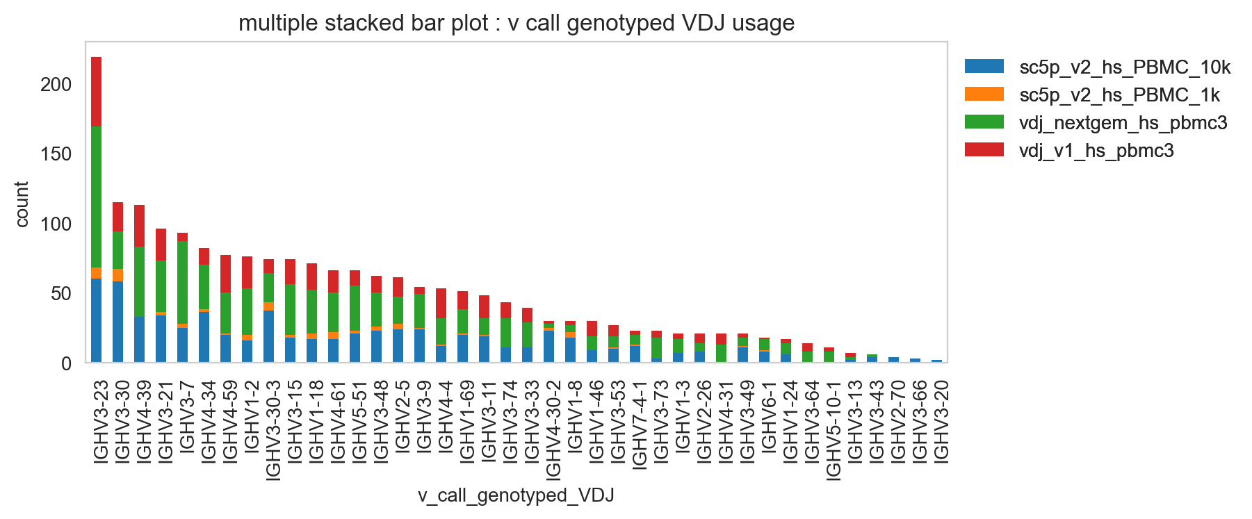
It’s obviously more useful if you don’t have too many groups, but you could try and plot everything and jiggle the legend options and color.
[24]:
ddl.pl.stackedbarplot(
    vdj_subset,
    color="v_call_genotyped_VDJ",
    groupby="sample_id",
)
plt.legend(bbox_to_anchor=(1, 1), loc="upper left", frameon=False)
plt.show()
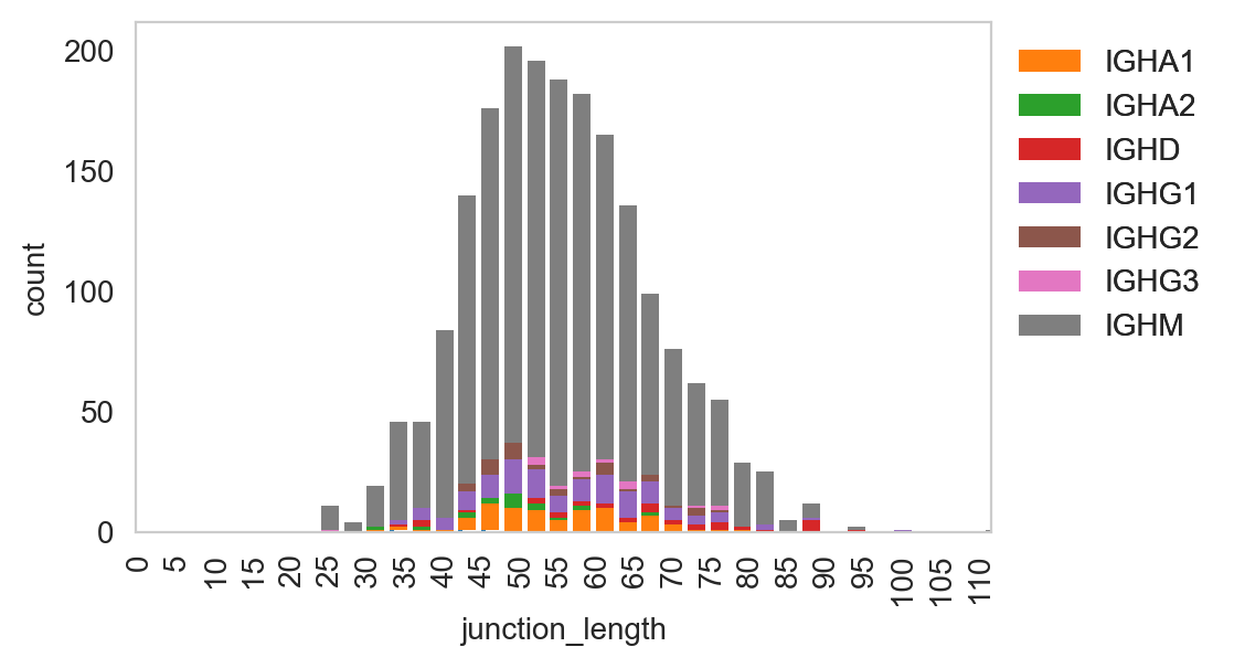
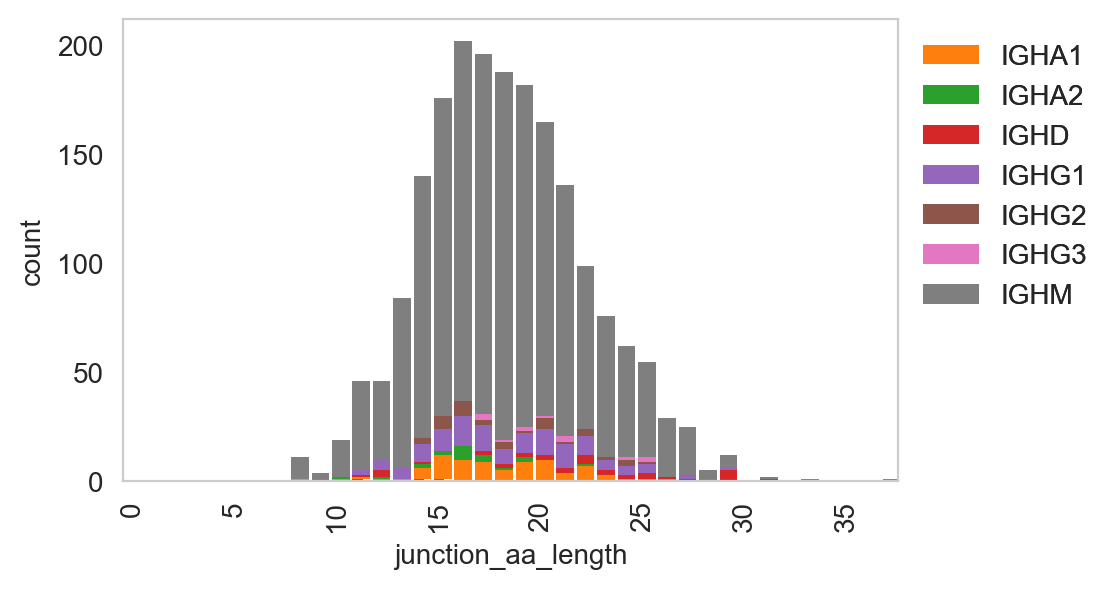
ddl.pl.spectratype
Spectratype plots contain info displaying CDR3 length distribution for specified groups. For this function, the current method only works for dandelion objects as it requires access to the contig-indexed .data slot.
[25]:
ddl.pl.spectratype(
    vdj_subset,
    color="junction_length",
    groupby="c_call",
    locus="IGH",
    width=2.3,
)
plt.legend(bbox_to_anchor=(1, 1), loc="upper left", frameon=False)
plt.show()
[26]:
ddl.pl.spectratype(
    vdj_subset,
    color="junction_aa_length",
    groupby="c_call",
    locus="IGH",
)
plt.legend(bbox_to_anchor=(1, 1), loc="upper left", frameon=False)
plt.show()
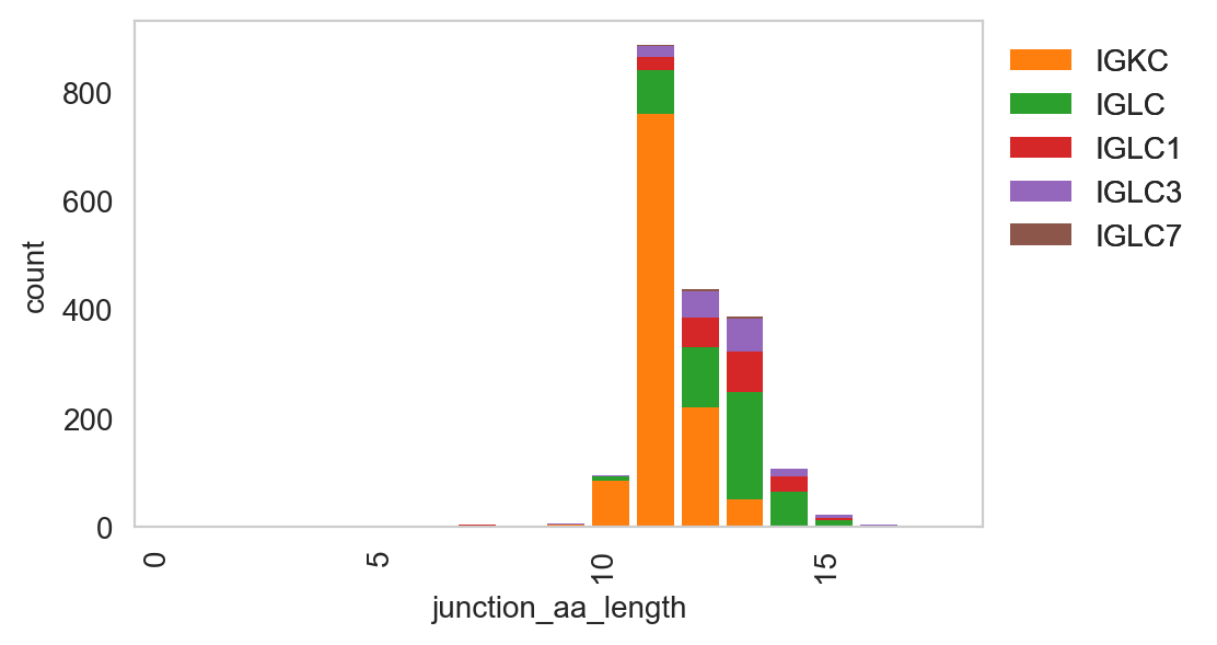
[27]:
ddl.pl.spectratype(
    vdj_subset,
    color="junction_aa_length",
    groupby="c_call",
    locus=["IGK", "IGL"],
)
plt.legend(bbox_to_anchor=(1, 1), loc="upper left", frameon=False)
plt.show()
ddl.pl.clone_overlap
There is now a circos-style clone overlap function where it looks for whather different samples share a clone. If they do, an arc/connection will be drawn between them.
[28]:
ddl.tl.clone_overlap(adata, groupby="leiden")
Finding clones
 finished: Updated AnnData:
   'uns', clone overlap table (0:00:00)
[29]:
sc.set_figure_params(figsize=[6, 6])
ddl.pl.clone_overlap(adata, groupby="leiden")
plt.show()
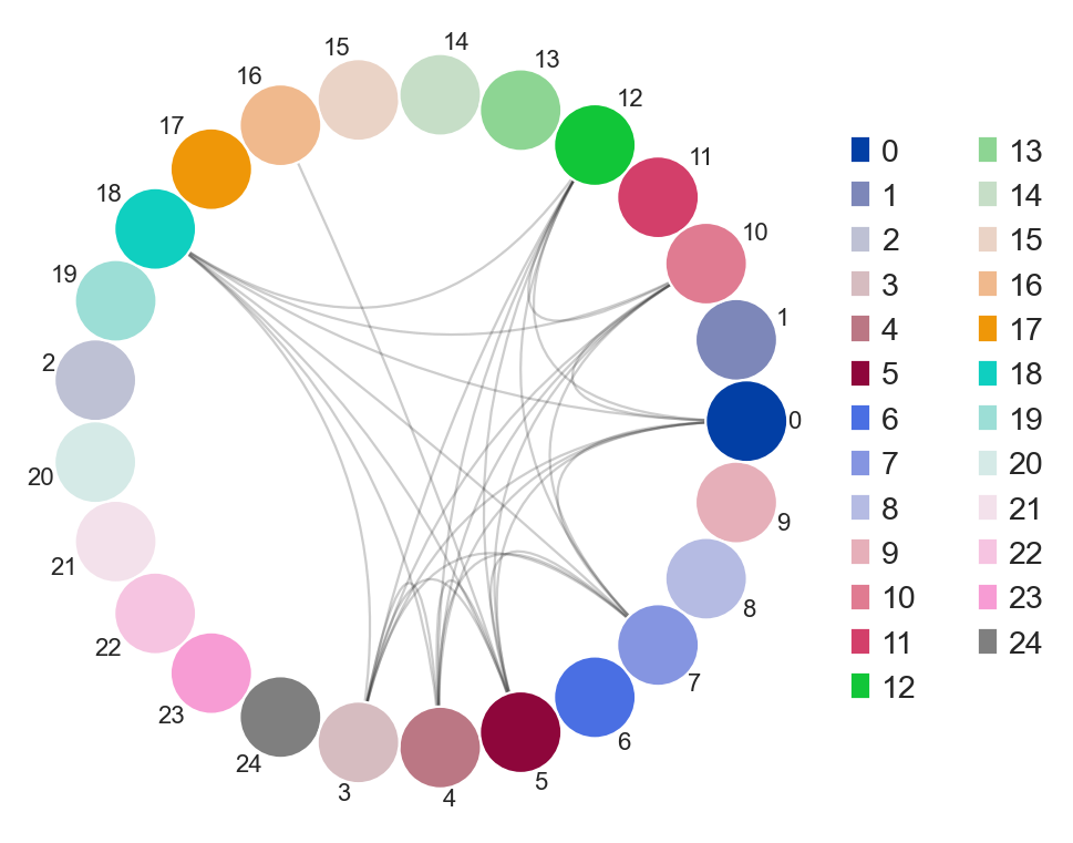
Other use cases for this would be, for example, to plot nodes as individual samples and the colors as group classifications of the samples. As long as this information is found in the .obs column in the AnnData, or even Dandelion.metadata, this will work.
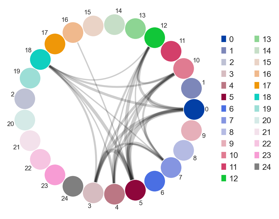
You an also specify weighted_overlap = True and the thickness of the edges will reflect the number of cells found to overlap between the nodes/samples.
[30]:
ddl.tl.clone_overlap(adata, groupby="leiden", weighted_overlap=True)
ddl.pl.clone_overlap(adata, groupby="leiden", weighted_overlap=True)
plt.show()
Finding clones
 finished: Updated AnnData:
   'uns', clone overlap table (0:00:00)
You can also specify colorby option. For example, if you provide a combined column to groupby, like group_leiden, you can specify group, leiden or group_leiden to colorby. Experiment around to see the different behaviour!
You can also visualise this as a heatmap by specifying as_heatmap = True.
[31]:
import seaborn as sns

sns.set(font_scale=0.8)

ddl.pl.clone_overlap(
    adata,
    groupby="leiden",
    weighted_overlap=True,
    as_heatmap=True,
    # seaborn clustermap kwargs
    cmap="Blues",
    annot=True,
    figsize=(8, 8),
    annot_kws={"size": 10},
    fmt="g",
)
plt.show()
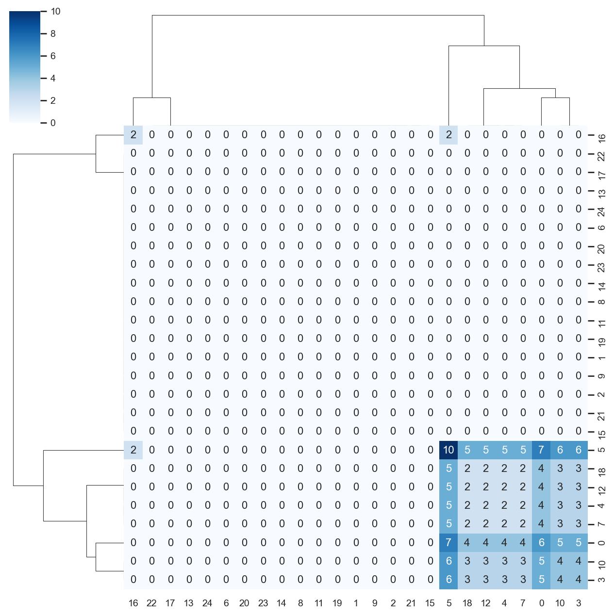
Note: colorby option with as_heatmap=True doesn’t do anything.
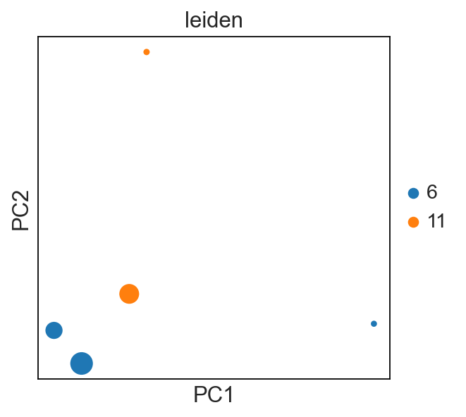
tl.vj_usage_pca
You can also compute the V/J gene usage in your various groups of interest. This function will return a new AnnData where instead of cells (obs) by gene (var), it will be groupby (obs) by V/J genes (var).
For example, I’m interested if the leiden clusters within each donor’s sample use V/J genes differently:
[32]:
# first make a concatenated group
adata.obs["sampleid_leiden"] = [
    s + "_" + l for s, l in zip(adata.obs["sampleid"], adata.obs["leiden"])
]
new_adata = ddl.tl.vj_usage_pca(
    adata,
    groupby="sampleid_leiden",
    mode="B",  # because B cells, use abT and gdT for alpha-beta and gamma-delta T cells respectively
    transfer_mapping=[
        "sampleid",
        "leiden",
    ],  # this transfers the sample_id and leiden values separately. if not provided, only sample_id_leiden is transferred.
    n_comps=3,  # 3 because the example is small here. the default is set at 30
)
new_adata
Computing PCA for V/J gene usage
computing PCA
    with n_comps=3
    finished (0:00:00)
 finished: Returned AnnData:
   'obsm', X_pca for V/J gene usage (0:00:00)
[32]:
AnnData object with n_obs × n_vars = 5 × 118
    obs: 'cell_type', 'cell_count', 'sampleid', 'leiden'
    uns: 'pca'
    obsm: 'X_pca'
    varm: 'PCs'
[33]:
sc.set_figure_params()

sc.pl.pca(new_adata, color="leiden", size=new_adata.obs["cell_count"])
# each dot is a `sample_id_leiden`. Check the .obs
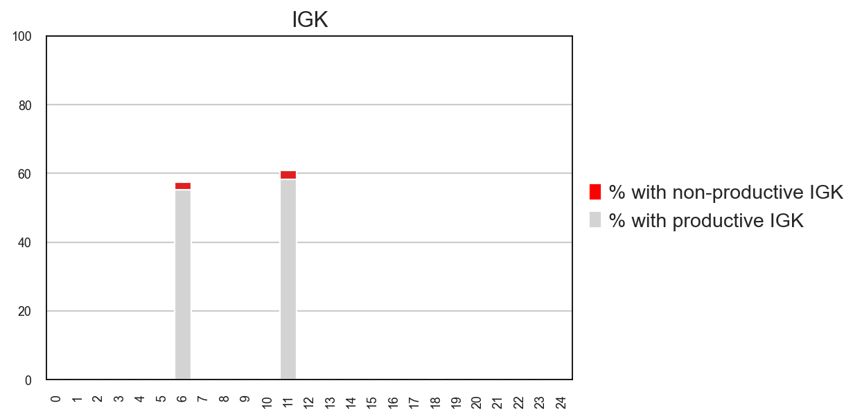
tl.productive_ratio/pl.productive_ratio
This new function lets you quantify what is the distribution of productive versus non-productive contigs at a cell-level. To do this, we need to re-check the Dandelion object so that non-productive columns are not removed.
[34]:
vdj2, adata2 = ddl.pp.check_contigs(vdj, adata, productive_only=False)
Filtering contigs
Preparing data: 5052it [00:00, 7936.51it/s]
Scanning for poor quality/ambiguous contigs: 100%|██████████| 2112/2112 [00:04<00:00, 443.71it/s]
Initializing Dandelion object
Transferring network
 finished: updated `.obs` with `.metadata`
 (0:00:00)
 finished: Returning Dandelion and AnnData objects:
 (0:00:06)
[35]:
ddl.tl.productive_ratio(adata2, vdj2, groupby="leiden", locus="IGK")
Tabulating productive ratio
 finished: Updated AnnData:
   'uns', productive_ratio (0:00:00)
[36]:
ddl.pl.productive_ratio(adata2, palette=["red", "lightgrey"])
plt.tight_layout()
# plt.savefig('plot.pdf')
plt.show()
[ ]: